Upload basin data
Provide the engineering inputs needed to derive HEC-HMS parameters for the basin.
Time series
Spatial layers
Read-only summary of the uploaded DEM. Upload a GeoTIFF (.tif) on the Upload Data tab to populate.
Global Soil Datasets
Two global soil rasters are clipped to Malaysia and shipped with the app — no upload required. These feed the Deficit & Constant loss method as fallback or primary inputs depending on what other data is available.
Hydrologic Soil Group (HYSOGs250m)
| What it is | USDA Hydrologic Soil Group (HSG) — A/B/C/D classification governing infiltration potential. Combines texture, drainage, depth-to-restrictive-layer per USDA NRCS NEH-630. |
|---|---|
| Source | Ross, C.W., Prihodko, L., Anchang, J., Kumar, S., Ji, W., & Hanan, N.P. (2018). Global Hydrologic Soil Groups (HYSOGs250m) for Curve Number-Based Runoff Modeling. ORNL DAAC, Oak Ridge, Tennessee, USA. |
| DOI |
10.3334/ORNLDAAC/1566
|
| Resolution | 250 m |
| Coverage in this app | Malaysia (clipped to national extent) |
| Native unit | Categorical (integer codes 1–4 for base groups, 11–14 for dual-class soils) |
| Distributor | NASA ORNL DAAC (free; NASA Earthdata Login required for global download) |
| Use in this app | Fallback Constant Rate (CR) estimate for D&C when texture data unavailable; SCS-Curve-Number input. Cross-check on texture-derived HSG when texture data IS available. |
Pixel-value encoding
| Code | HSG | Description |
|---|---|---|
| 1 | A | Low runoff potential (>90% sand and <10% clay) |
| 2 | B | Moderately low runoff potential (50–90% sand, 10–20% clay) |
| 3 | C | Moderately high runoff potential (<50% sand, 20–40% clay) |
| 4 | D | High runoff potential (<50% sand, >40% clay) |
| 11 | A/D | High runoff potential unless drained — texture A but shallow water table |
| 12 | B/D | High runoff potential unless drained — texture B but shallow water table |
| 13 | C/D | High runoff potential unless drained — texture C but shallow water table |
| 14 | D/D | High runoff potential always (deeply drained or not) |
Dual-class /D codes: treat as the base letter (A/B/C/D) when artificial drainage is in place; treat as D when undrained. HEC-HMS users typically pick one interpretation per project.
HSG → Constant Rate fallback table
Used when no texture data is available. Per HEC TRM / Saleh et al. (2011) ranges (narrower, conservative) and Cahyono & Adidarma (2019) / Sahu et al. (2023) ranges (wider, sensitivity check).
| HSG | Soil description | CR (mm/hr) — HEC TRM | CR (mm/hr) — Cahyono & Adidarma |
|---|---|---|---|
| A | Deep, well-drained sands/gravels | 7.62–11.43 | >36.1 |
| B | Moderately deep, well-drained (Loam) | 3.81–7.62 | 14.5–36.1 |
| C | Layers impeding drainage (Clay Loam) | 1.27–3.81 | 1.5–14.5 |
| D | High clay, shallow, or high water table | 0–1.27 | <1.5 |
HSG decision tree note: Texture is the primary driver of HSG, but USDA NRCS also factors in (1) depth to impermeable layer / bedrock — if shallow (<50 cm), automatically D regardless of texture; and (2) depth to water table — if shallow, soil gets a /D dual class. Texture-only HSG approximations miss factors (1) and (2); HYSOGs250m runs the full decision tree.
Depth to Bedrock (mm) (BDRICM)
| What it is | Soil depth from the surface to the R horizon (where soil ends and consolidated bedrock begins). In HEC-HMS Deficit & Constant, this is the active soil layer depth Z used in D_init = (θ_sat − θ_init) × Z and D_max = (θ_sat − θ_wp) × Z. |
|---|---|
| Source | Shangguan, W., Hengl, T., Mendes de Jesus, J., Yuan, H., & Dai, Y. (2017). Mapping the global depth to bedrock for land surface modeling. Journal of Advances in Modeling Earth Systems, 9(1), 65–88. |
| DOI |
10.1002/2016MS000686
|
| Resolution | 250 m |
| Coverage in this app | Malaysia (clipped to national extent) |
| Native unit | Centimetres (this app: pre-converted to millimetres before bundling — see app's `data/precomputed/bdricm/bdricm_mm_cog.tif`) |
| Range in this app | 540 mm to 2000 mm (Malaysia clip) |
| Cap interpretation | Pixels at 2000 mm mean ≥ 2 m of soil , not exactly 2 m. Shangguan et al. capped the raster at 200 cm = 2000 mm because prediction uncertainty grows beyond 2 m. For Malaysian lowland sub-basins, expect most cells at the cap. |
| Distributor | ISRIC legacy archive (1.4 GB global GeoTIFF; this app ships a 4.3 MB Malaysia-clipped COG) |
| Note on SoilGrids version | NOT part of SoilGrids v2.0 (Poggio et al. 2021). Lives in the legacy 2017 archive. Often cited as 'SoilGrids250m – Depth to bedrock' (e.g., Moumni et al. 2021); same data either way. |
| Use in this app | Per-sub-basin Z via zonal mean. Feeds D_init and D_max equations directly. Replaces the older convention of a single global Z (RASHMS guidance 300–600 mm) with spatially-varying Z. |
Citations & further reading
- Ross, C.W., et al. (2018). Global Hydrologic Soil Groups (HYSOGs250m) for Curve Number-Based Runoff Modeling. ORNL DAAC . https://doi.org/10.3334/ORNLDAAC/1566
- Shangguan, W., Hengl, T., Mendes de Jesus, J., Yuan, H., & Dai, Y. (2017). Mapping the global depth to bedrock for land surface modeling. Journal of Advances in Modeling Earth Systems , 9(1), 65–88. https://doi.org/10.1002/2016MS000686
- Moumni, H., Sebari, K., Stour, L., & Ahbari, A. (2021). Estimation of the HEC-HMS model parameters in data-scarce regions: Application to the Ouergha watershed (Sebou, Morocco). E3S Web of Conferences , 314, 05002 — uses BDRICM as Z source per sub-basin.
- USDA NRCS (2009). National Engineering Handbook, Part 630, Chapter 7 — Hydrologic Soil Groups.
- HEC TRM — Hydrologic Modeling System Technical Reference Manual; HSG → CR ranges.
Why pre-bundled? Both rasters are global products that don't change between projects. Clipping once to Malaysia and shipping with the app means engineers can model any Malaysian basin without manually downloading from ORNL DAAC / ISRIC each time. Storage cost: ~5 MB total.
Derive the longest flowpath per sub-basin (fill → D8 pointer → D8 flow accumulation → rasterise basins → longest flowpath). Outputs length, upstream + downstream elevation, and average slope. Polylines render on the Basin Map; results feed Overall Characteristics.
Pre-requisites
Refine specific sub-basins
If a flowpath line looks wrong (cuts a ridge, ends at the wrong outlet), select that sub-basin and re-run only it. The new line replaces the existing one.
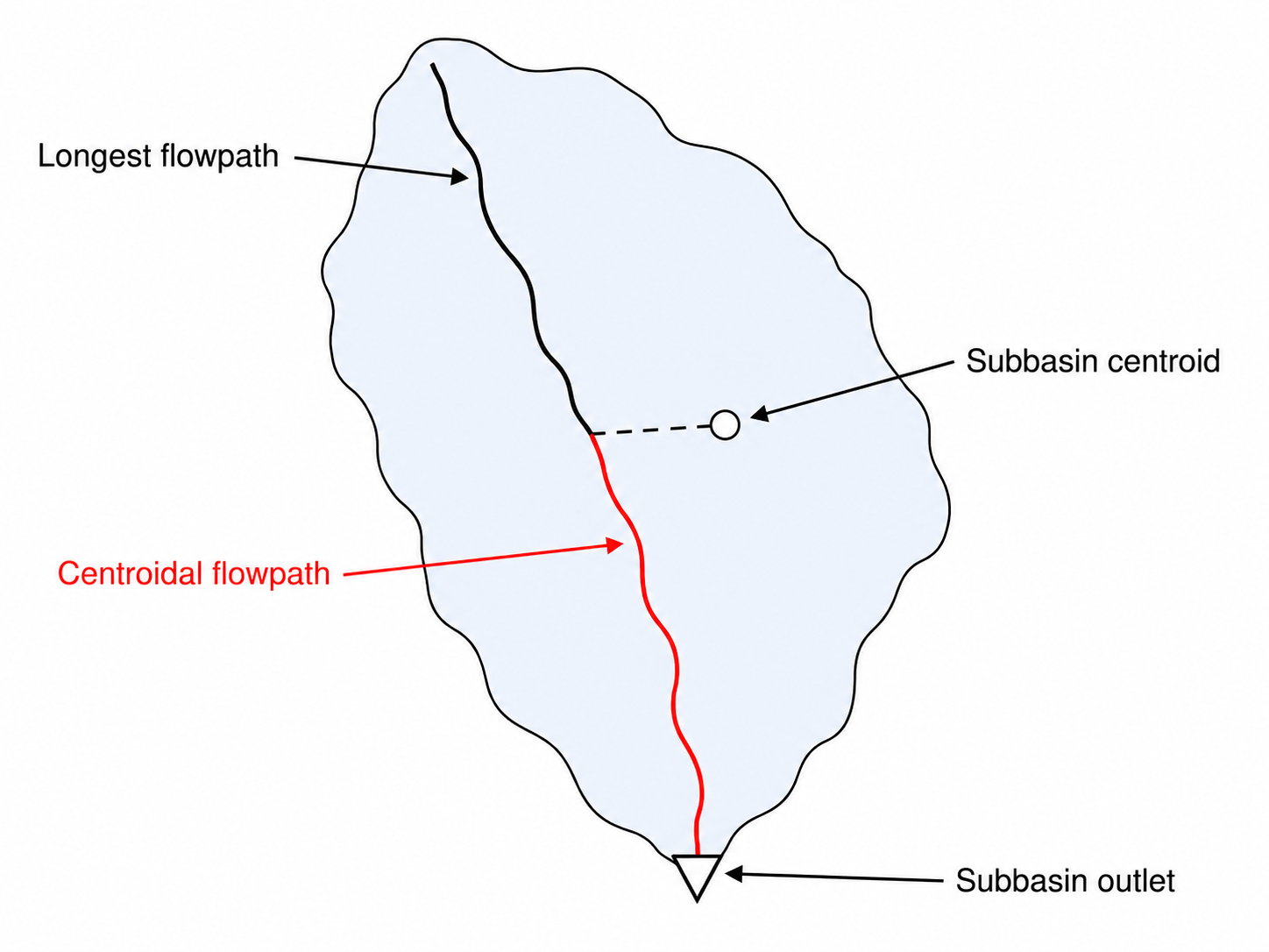
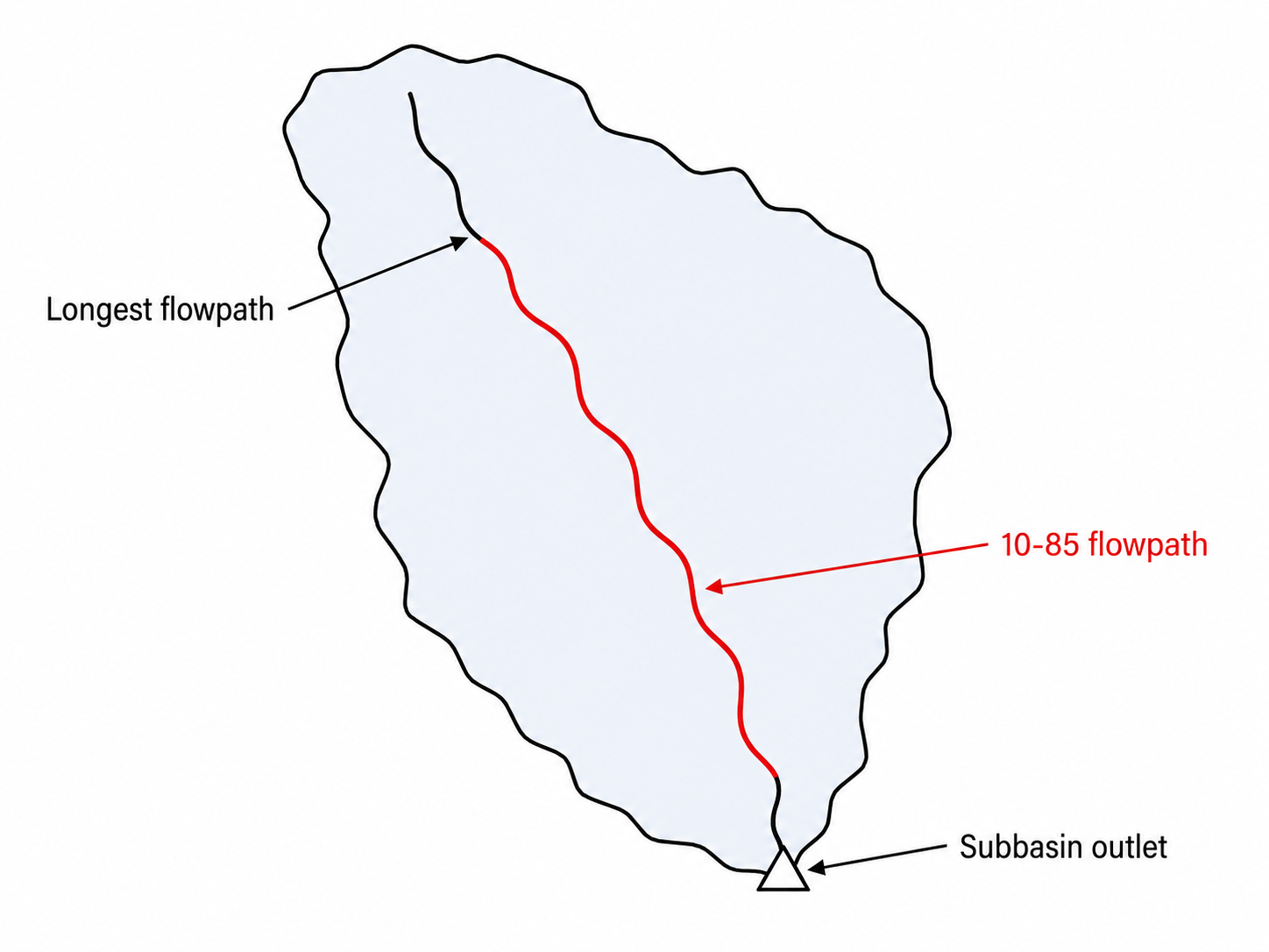
Centroidal & 10-85 Flowpath
Derives the centroidal flowpath (outlet → projection of basin centroid onto the longest flowpath) and the 10-85 flowpath (segment between the 10% and 85% length points measured upstream from the outlet). Lengths in km, slopes in m/m. Polylines render on the map as separate layers (green = centroidal, orange = 10-85). Re-running Longest Flowpath clears these results.
-
BASIN— basin ID (matches the rasterised basin index) -
LENGTH— longest flow-path length (m) -
UP_ELEV— upstream channel elevation (m) -
DN_ELEV— downstream channel elevation (m) -
AVG_SLOPE— average slope along the flow path (%)
Slope conversion: m/m = % / 100.
Centroidal Flowpath
Segment of the longest flowpath from the outlet to the point where the basin centroid projects onto it. Used by SCS lag-time and Snyder unit-hydrograph methods.
10-85 Flowpath
Segment of the longest flowpath between the 10% and 85% length points measured upstream from the outlet. Slope of this segment feeds USGS regression equations (e.g., Texas, Florida).
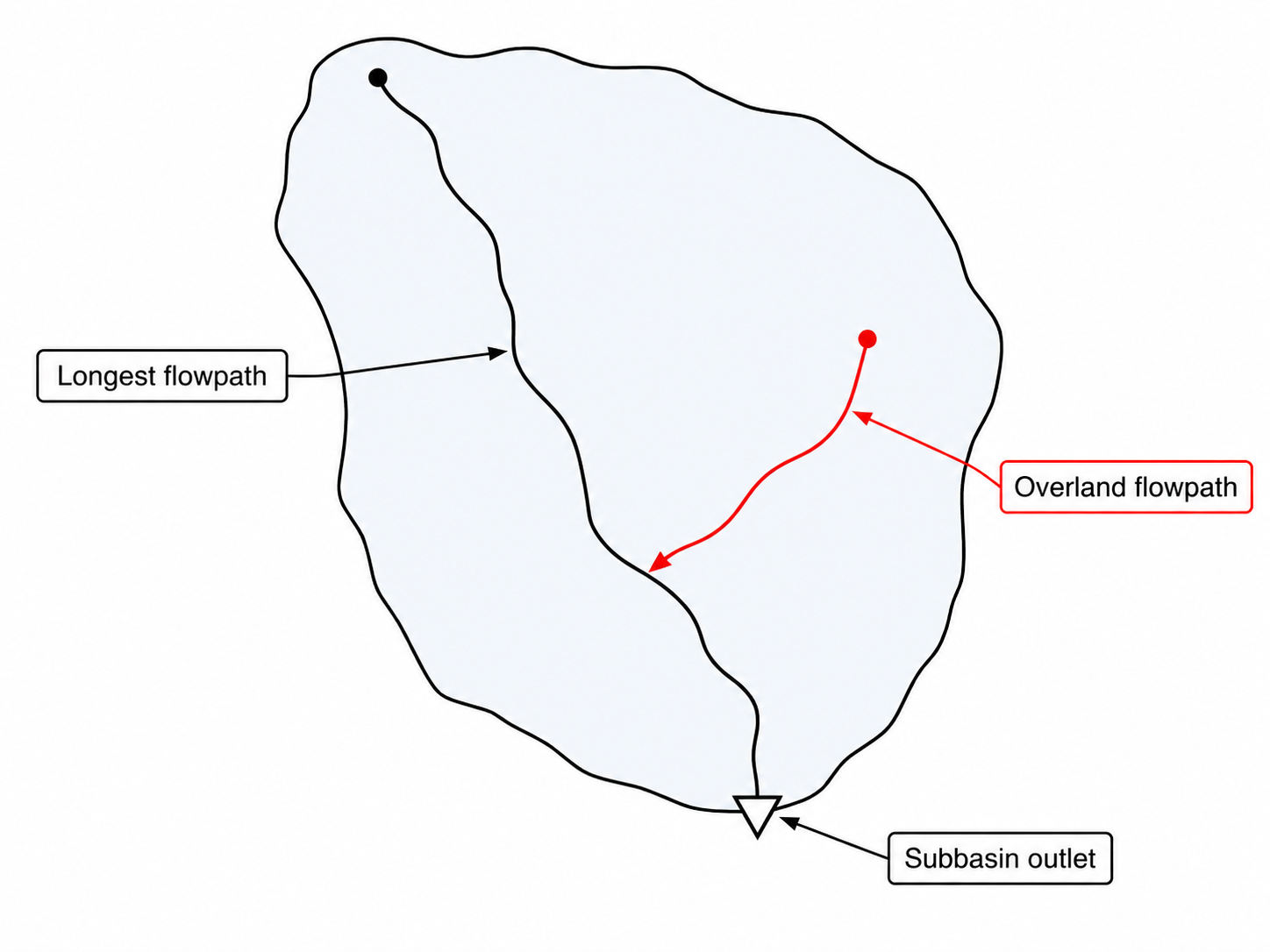
Derives the overland (sheet-flow) length and slope per sub-basin by walking each longest flowpath from the upstream end to where it first meets a defined stream channel. The stream channel is recognised wherever the DEM's flow accumulation exceeds the configured threshold. Outputs feed the Kerby and Kerby-Kirpich Tc methods downstream.
Pre-requisites
- L = longest flowpath − stream network
- Sheet flow ends where channel forms
- "end the sheet flow segment at that physical point"
- L between 30–366 m: use Kerby normally
- L > 366 m: clip to 366 m (Kerby cap), excess → Kirpich channel
- L very small but > 0: use anyway (no minimum)
- L = 0 (channel from divide): drop Kerby, use Kirpich alone
Overland Flowpath schematic
Compute area-weighted SCS Curve Number per sub-basin from the engineer's per-class lookup of CN values. Outputs: CN, CN Canonical (Malaysia), Upper CN (ARC III), Lower CN (ARC I).
Pre-requisites
Step 1 — HSG source
HSG ADOPTED = engineer-uploaded soil polygons + per-class HSG lookup. HYSOGs250m = bundled Ross et al. (2018) global 250 m raster, clipped to Malaysia (no soil upload needed).
Codes 11=A/D, 12=B/D, 13=C/D, 14=D/D. Drained = base letter. Undrained = collapse all dual codes to D.
Step 2 — Per-class lookup
One row per unique uploaded LULC class. Pick a Type from the Landuse class dropdown — CN A / B / C / D / Canonical (Malaysia) auto-fill from the CN ADOPTED reference. You can also override any numeric cell directly. Green ✓ = mapped; yellow ⚠ = no mapping (pick a Type or fill the CN cells manually).
One row per unique uploaded soil class. Pick a Type from the Soil class dropdown — the HSG group letter (A/B/C/D) auto-fills from the HSG ADOPTED reference. You can also override the HSG group dropdown directly. Green ✓ = mapped; yellow ⚠ = no mapping.
Step 3 — Run
Weight each landuse × HSG zone by its area within the sub-basin.
CN_j = Σ (CN_i · A_i) / Σ A_i
       where  i  = each landuse × HSG zone inside sub-basin j
              CN_i = TR-55 CN at that zone's HSG group
              A_i  = zone area (km²)
Reference: USDA-NRCS TR-55 (1986), Urban Hydrology for Small Watersheds
2. Potential maximum retention
S = 25400 / CN − 254      [S in mm]
S = 1000 / CN − 10         [S in inches]
Initial abstraction: I_a = 0.2 · S  (default; calibratable 0.05 S – 0.15 S)
Reference: SCS National Engineering Handbook (NEH), Part 630, Chapter 10.
3. ARC I / ARC III moisture bands (Upper CN / Lower CN)
Adjust the AMC-II (average) CN to dry (ARC I) and wet (ARC III) conditions. Used as the Lower CN / Upper CN sensitivity envelope in the Results table. Hawkins (1985) reciprocal form as adopted in NRCS NEH-630.
Lower CN = CN_I  = 4.2 · CN_II / (10 − 0.058 · CN_II)        (dry)
Upper CN = CN_III = 23  · CN_II / (10 + 0.13  · CN_II)        (wet)

Check  (CN_II = 80): CN_I = 62.7,  CN_III = 90.2
- USDA-NRCS, NEH Part 630, Chapter 10 (2004), Eq. 10-13 + 10-14, Table 10-1
- Hawkins, R.H. (1985) A comparison of predicted and observed runoff curve numbers , in Proc. ASCE Specialty Conf. on Watershed Management
- Mishra, S.K. & Singh, V.P. (2003) Soil Conservation Service Curve Number (SCS-CN) Methodology , Springer, Eq. 2.49-2.52
- Hawkins, R.H. et al. (2009) Curve Number Hydrology: State of the Practice , ASCE-EWRI
4. Hydrologic Soil Groups (HSG)
USDA categorises soils by minimum infiltration rate:
A: > 0.30 in/hr  — sand, loamy sand, sandy loam      (low runoff)
B: 0.15-0.30 in/hr — silt loam, loam                  (moderate)
C: 0.05-0.15 in/hr — sandy clay loam                   (high)
D: < 0.05 in/hr  — clay loam, silty clay, clay         (very high)
Reference: USDA-NRCS, National Engineering Handbook, Part 630, Chapter 7 (2007).
5. HYSOGs250m (bundled global HSG raster)
Ross, C.W., Prihodko, L., Anchang, J., Kumar, S., Ji, W.,
Hanan, N.P. (2018).
Global Hydrologic Soil Groups
(HYSOGs250m) for Curve Number-Based Runoff Modeling
.
ORNL DAAC, Oak Ridge, TN, USA. DOI:
10.3334/ORNLDAAC/1566
.
Pixel encoding — 1=A, 2=B, 3=C, 4=D, 11=A/D, 12=B/D, 13=C/D, 14=D/D.
6. Adopted Curve Number (Malaysia Condition) — Canonical column
33 land-use categories with single AMC-II CN values adopted for Malaysian conditions (HSG-independent). Source: DID Malaysia HP standards + practitioner consensus (From Ruzaimie).
7. TR-55 example CN tables
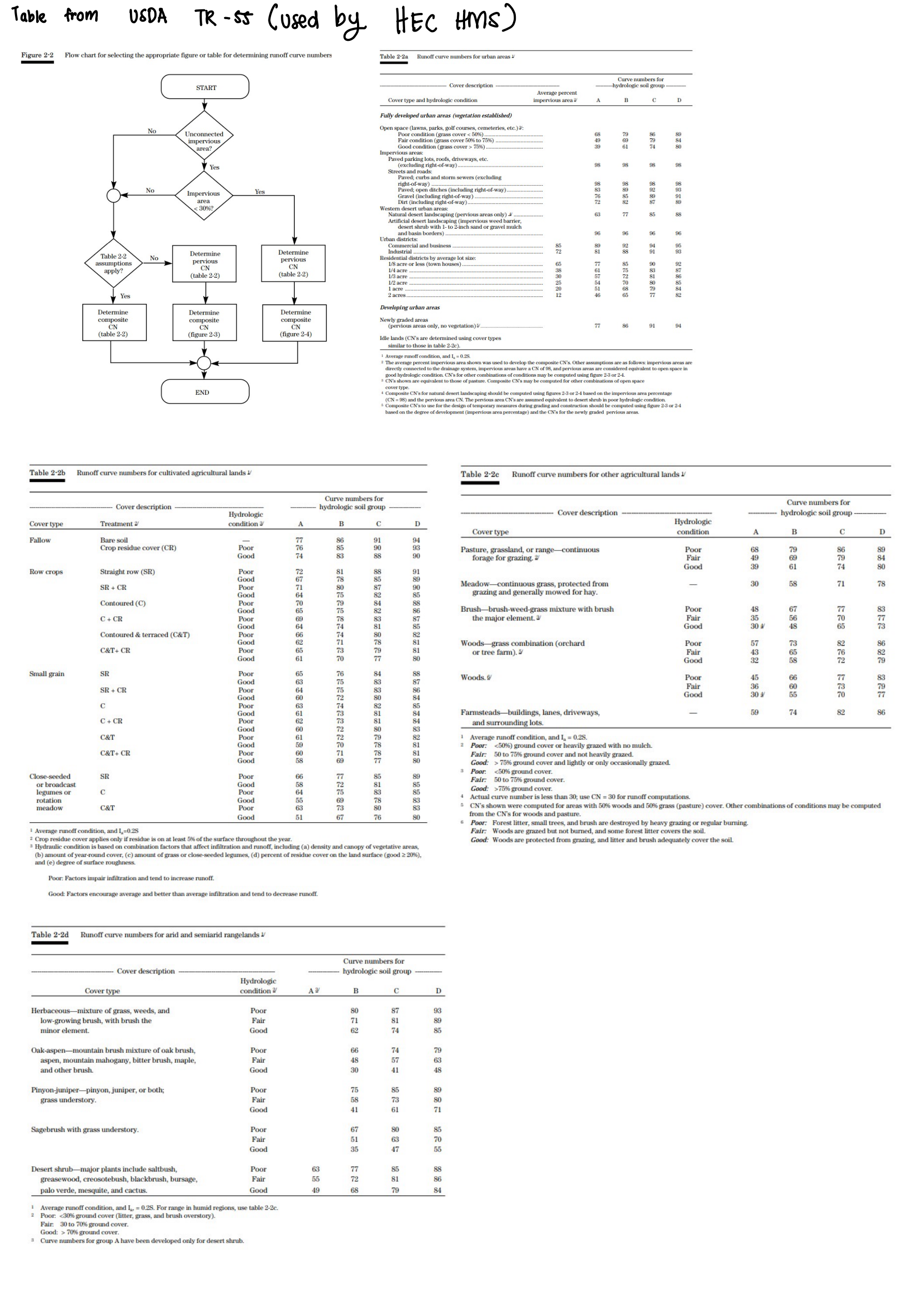
USDA-SCS (1986) TR-55, Urban Hydrology for Small Watersheds, 2nd ed., Tables 2-2a (urban), 2-2b (cultivated agricultural), 2-2c (other agricultural), 2-2d (arid/semiarid rangelands).
8. HSG ADOPTED reference table
Soil texture → HSG group mapping bundled with the app. Source for the auto-fill on the Soil per-class lookup and the 📖 reference modal in the Curve Number User-Defined panel.
9. CN ADOPTED reference table (multi-HSG)
Land-use class → CN per HSG (A/B/C/D) + Canonical (Malaysia) column. Source for the auto-fill on the LU per-class lookup and the 📖 reference modal in the Curve Number User-Defined panel.
Compute area-weighted Kerby retardance N per sub-basin. Used by Kerby + Kerby-Kirpich Tc methods on the Tc/Tp tab. Pick a canonical Kerby surface for each uploaded LULC class — N cascades from the bundled Kerby 1959 / Roussel 2005 table.
Pre-requisites
Per-class lookup
One row per unique uploaded LULC class. Pick a canonical surface from the dropdown (6 options); the N value cascades from the bundled table. Engineer can override the N cell directly (per Kerby 1959 — don't interpolate between rows, but deliberate override IS allowed). Green ✓ = mapped; yellow ⚠ = no mapping (pick a surface or set N manually).
Run
Kerby 1959 / Roussel et al. 2005. Don't interpolate N — pick the row matching the surface. Override individual rows in the per-class table if needed.
| Surface | N | Source |
|---|---|---|
| Pavement | 0.02 | Kerby 1959 / Roussel 2005 |
| Smooth bare packed soil | 0.10 | Kerby 1959 |
| Poor grass, cultivated row crops, moderately rough packed surfaces | 0.20 | Kerby 1959 |
| Average grass / pasture | 0.40 | Kerby 1959 |
| Deciduous forest | 0.60 | Kerby 1959 |
| Dense grass, coniferous forest, or deciduous forest with deep litter | 0.80 | Kerby 1959 |
2. Area-weighted N per sub-basin
Weight each LULC zone by its area within the sub-basin.
N_j = Σ (N_i · A_i) / Σ A_i
       where  i  = each LULC zone inside sub-basin j
              N_i = Kerby N at that zone's canonical surface
              A_i  = zone area (km²)
3. Why Kerby N ≠ Manning's n ≠ Izzard Cr
Three different empirical methods, three different parameter conventions for surface retardance. Kerby N (this tab) uses 0.02-0.80; Manning's n (overland) uses 0.011-0.80 but lower for smooth surfaces; Izzard Cr uses 0.007-0.060. Not interchangeable. Never substitute one for another.
4. Methods that consume this output
- Kerby (1959): T_o = K · (N · L)^0.467 · S^(−0.235), L ≤ 366 m (1,200 ft cap)
- Kerby-Kirpich combined: T_c = T_o (Kerby overland) + T_ch (Kirpich channel) — Roussel 2005 preferred Texas implementation
5. Citations
- Kerby, W.S. (1959). Time of concentration for overland flow. Civil Engineering 29(3), 174.
- Roussel, M.C., Thompson, D.B., Fang, X., Cleveland, T.G., & Garcia, C.A. (2005). Time-Parameter Estimation for Applicable Texas Watersheds. TxDOT Research Report 0-4696-2.
- FHWA (2009). Urban Drainage Design Manual (Hydraulic Engineering Circular No. 22, HEC-22, 3rd ed.).
- Hathaway, G.A. (1945). Design of drainage facilities for military airfields. Trans. ASCE 110, 697.
Compute area-weighted Rational Runoff Coefficient C per sub-basin. Used by FAA Tc method + Rational Q = C·i·A peak flow (HP 5 workflow). Pick a canonical HEC-22 cover type for each uploaded LULC class — C cascades from the midpoint of the HEC-22 Table 3-1 published range.
Pre-requisites
Per-class lookup
One row per unique uploaded LULC class. Pick a HEC-22 cover from the dropdown (19 options); the C value cascades from the midpoint of the published range. Engineer can override the C cell directly (e.g. to bias toward the higher end of the range for steeply sloped areas / longer return periods, per the HEC-22 footnote).
Run
FHWA HEC-22 (3rd ed., 2009) Urban Drainage Design Manual, Chapter 3, Table 3-1. Verified against original publication. The C column is the midpoint of the published range, used as the dropdown cascade default; engineer can override per row.
HEC-22 footnote: "Higher values are usually appropriate for steeply sloped areas and longer return periods because infiltration and other losses have a proportionally smaller effect on runoff in these cases."
| Type of Drainage Area | C min | C max | C (midpoint) |
|---|---|---|---|
| Business — Downtown | 0.70 | 0.95 | 0.83 |
| Business — Neighborhood | 0.50 | 0.70 | 0.60 |
| Residential — Single-family | 0.30 | 0.50 | 0.40 |
| Residential — Multi-units, detached | 0.40 | 0.60 | 0.50 |
| Residential — Multi-units, attached | 0.60 | 0.75 | 0.68 |
| Residential — Suburban | 0.25 | 0.40 | 0.33 |
| Residential — Apartment dwelling | 0.50 | 0.70 | 0.60 |
| Industrial — Light | 0.50 | 0.80 | 0.65 |
| Industrial — Heavy | 0.60 | 0.90 | 0.75 |
| Parks, cemeteries | 0.10 | 0.25 | 0.18 |
| Playgrounds | 0.20 | 0.40 | 0.30 |
| Railroad yard | 0.20 | 0.40 | 0.30 |
| Unimproved areas | 0.10 | 0.30 | 0.20 |
| Lawns (avg, combined sandy/heavy soil, 2-7% slope) | 0.10 | 0.22 | 0.16 |
| Streets — Asphaltic | 0.70 | 0.95 | 0.83 |
| Streets — Concrete | 0.80 | 0.95 | 0.88 |
| Streets — Brick | 0.70 | 0.85 | 0.78 |
| Drives and walks | 0.75 | 0.85 | 0.80 |
| Roofs | 0.75 | 0.95 | 0.85 |
Lawns row collapses HEC-22's original 6 sub-rows (Sandy × {flat, avg, steep} + Heavy × {flat, avg, steep}) into a single "average slope" entry — soil texture × slope info isn't carried per-polygon in typical LULC shapefiles, so the finer breakdown adds no actionable granularity. Range shown is the average-slope band of Sandy + Heavy combined.
2. Area-weighted C per sub-basin
Weight each LULC zone by its area within the sub-basin (standard Rational compound-coefficient method).
C_j = Σ (C_i · A_i) / Σ A_i
       where  i  = each LULC zone inside sub-basin j
              C_i = HEC-22 Rational C at that zone's cover type
              A_i = zone area (km²)
3. Methods that consume this output
- FAA Tc (1970): T_c = 1.8 · [(1.1 − C) · L_c^0.5 / S_c^(1/3)]
- Rational peak flow (Q = C·i·A): used in HP 5 Malaysia design flood workflow + standalone Rational Method applications
4. Why Rational C ≠ Curve Number ≠ Kerby N
Rational C (this tab) is a dimensionless runoff fraction (0-1). Curve Number (CN tab) is the SCS retention parameter with a different physical basis. Kerby N (separate tab) is a surface retardance coefficient. Not interchangeable. Each feeds its own family of Tc / loss methods.
5. Citations
-
FHWA (2009).
Urban Drainage Design Manual
(HEC-22, 3rd ed., Publication No. FHWA-NHI-10-009).
Federal Highway Administration. Available:
https://www.fhwa.dot.gov/engineering/hydraulics/pubs/10009/ - ASCE / WEF (1992). Design and Construction of Urban Stormwater Management Systems (ASCE Manual of Practice No. 77 / WEF Manual of Practice FD-20). American Society of Civil Engineers + Water Environment Federation.
- Chow, V.T., Maidment, D.R., & Mays, L.W. (1988). Applied Hydrology . McGraw-Hill. Table 15.1.1 reproduces the ASCE/HEC-22 Rational C values for textbook use.
- FAA Advisory Circular 150/5320-5B (1970) — original FAA drainage design source for the Tc form that consumes this C.
Compute total impervious percentage per sub-basin. Tick the LULC class values from your uploaded shapefile that are impervious. The app sums their area within each sub-basin and divides by sub-basin area. Used by HEC-HMS as the "Percent Impervious" sub-basin input (every Loss Method treats impervious area as 100% runoff bypassing infiltration).
Pre-requisites
Step 1 — Tick impervious LULC classes
First load: auto-ticked by a regex heuristic (Pavement / Built / Commercial / Industrial / Water bodies). Review + adjust manually below. Map preview "Impervious preview" on the Basin Map highlights what's selected in red — toggle it on to sanity-check.
Step 2 — Run
The HEC-HMS subbasin element editor has a "Percent Impervious" field — one value per sub-basin, range 0-100. This field is applied by EVERY Loss Method (SCS-CN, Deficit & Constant, Initial & Constant, Green & Ampt): the impervious fraction of the sub-basin generates 100% runoff bypassing the loss method's infiltration calculation. The remaining (pervious) fraction is routed through the loss method normally.
Reference: HEC-HMS Technical Reference Manual, Loss chapter; HEC-HMS User's Manual, Subbasin Elements section.
2. Compute formula
Impervious_j (%) = 100 · Σ(A_i · I_i) / Σ A_i
       where  i  = each LULC zone inside sub-basin j
              I_i = 1 if class is ticked, 0 otherwise
              A_i = zone area (km²)
3. Auto-tick heuristic (default for first load)
On first load (no engineer selection yet) the following case-insensitive regex patterns are pre-ticked against uploaded class names. Engineer reviews + adjusts.
-
pavement | paved | asphalt | concrete -
street | road | highway | drive | walk -
railway | rail-road | train | transport | airport | runway -
roof | building.roof -
built | urban | downtown | business | commercial -
industrial | factory | warehouse -
high-rise | apartment | condo | flat -
infrastructure | utility -
water | river | lake | pond | reservoir | sea | ocean | aquaculture | waterbody— water surface = 100% runoff per Rational Method convention
4. What's NOT pre-ticked by heuristic
- Forest / Tree cover / Oil Palm / Rubber / Coconut / Cocoa
- Paddy / Crops / Agricultural / Horticulture / Orchard
- Grassland / Pasture / Herbaceous / Shrubland / Mangrove / Swamp
- Bare land / Cleared / Landfill / Quarry / Mining (no canopy but still infiltrates)
- Residential — auto-ticked ONLY for keywords like "residential.urban" or "high-rise"; generic "Residential" is left unticked because rural residential in Malaysia is mostly kampung (large pervious yards, low impervious)
Default behaviour can over-simplify mixed-use classes like "Residential" (which is genuinely ~35% paved in dense suburbs). Override per-row in the Results table if your basin has substantial mixed-use LULC.
5. Sanity check via map preview
Toggle the "Impervious preview" layer on the Basin Map to see the LULC polygons currently ticked as impervious — they render in red. Useful for catching obviously-wrong selections (e.g. a forest class wrongly auto-ticked because its name happens to contain "road").
6. Related
- Curve Number (CN tab) — TR-55 Table 2-2a indirectly bakes in impervious % for urban residential categories; this tab is the standalone Impervious value HEC-HMS expects as a separate sub-basin input.
- Surface Method tab — "paved classes" selection there serves a different purpose (Max Canopy = 0 for paved); not coupled to this tab's selection by design.
Compute Time of Concentration per sub-basin. Tick any subset of the 10 methods, pick one as Primary (feeds Overall Characteristics), assign flowpaths per method as needed. Methods auto-pull L / Lc / S / A / CN / N / C from upstream Basin Characteristics tabs.
Pre-requisites
Step 1 — Pick methods (Tick = compute · Primary = Overall Char source)
Step 2 — Per-method equation + flowpath assignment
Step 3 — Run
Cross-method summary
Best-for / avoid-when guidance for each method, sourced from 43 peer-reviewed references.
2. Flowpath glossary
- Longest flowpath — from Longest Flowpath tab; the longest hydraulic path divide → outlet. Used as L for channel / main-stream-dominated methods (Kirpich, HP 5, HP 27, Bransby-Williams, NRCS Lag-time, USACE).
- Overland flowpath — from Overland Flowpath tab; the sheet-flow portion from upstream end to channel-start. Used by Kerby + FAA (overland-dominated methods).
- Centroidal flowpath — from Centroidal & 10-85 sub-section; outlet → centroid projection on the longest flowpath. Used as L_c by USACE Mainstem Columbia.
- 10-85 flowpath — from Centroidal & 10-85 sub-section; segment between 10% and 85% length points (upstream from outlet). Slope of this segment feeds USACE Mainstem Columbia.
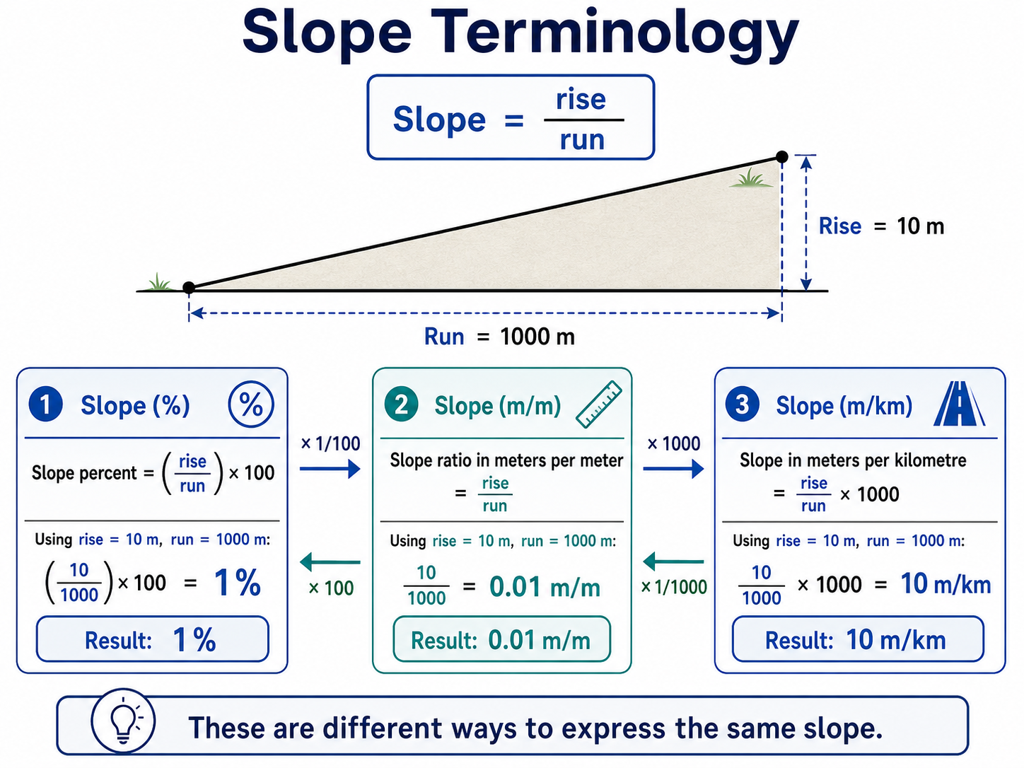
3. Slope terminology — three equivalent expressions
All three lines below describe the SAME slope. Worked example: rise = 10 m over run = 1000 m → 1% = 0.01 m/m = 10 m/km .
4. S unit required per method (cross-method quick lookup)
Each method's regression coefficient assumes a specific S unit. Pick the matching slope dropdown flavour in the equation card; the % vs m/m vs m/km mismatches produce 10×–1000× Tc errors silently.
- m/m decimal — Kirpich, Kerby, Kerby-Kirpich
- % (full number, e.g. 3 not 0.03) — HP 5, FAA, NRCS Lag-time
- m/km — HP 27, Bransby-Williams, USACE Mainstem Columbia
- none — Sanity Check (area-only, no slope input)
5. HEC-HMS transform field mapping (downstream)
Where the Tc you compute here plugs into the Transform tab.
- Clark UH Time of Concentration : hours
-
Clark UH
Storage Coefficient (R)
:
hours
— ratio
R/(R+Tc)≈ 0.5–0.7 typical. - SCS UH Lag : minutes (Lag ≠ Tc — apply Lag = 0.6 × Tc)
- Snyder UH Standard Lag : hours
Compute Lag Time per sub-basin. Tick any subset of 6 methods, pick one as Primary. Methods 1, 6, 7 (SCS Lag, Roussel, McCuen) consume Tc — by default the Primary Tc from the Tc tab; override per method via dropdown.
Pre-requisites
Step 1 — Pick methods
Step 2 — Per-method equation + flowpath / Tc source assignment
Step 3 — Run
Cross-method summary
Best-for / avoid-when guidance for each Lag method, sourced from peer-reviewed literature.
2. Critical rule — DO NOT double-apply the 0.6 factor
Methods that output
lag directly
(HP 11, Carter, Eagleson, McCuen as L_H, Roussel as T_L)
must be entered as-is into HEC-HMS Lag fields. Applying
× 0.6
on top of an already-lag value
underestimates lag by 40%
— the single most common entry error.
Compute Thiessen-weighted areal rainfall for every sub-basin in the uploaded basin shapefile, then dedup identical series so each HEC-HMS sub-basin can reference a single gauge per unique rainfall input.
Pre-requisites
Thiessen (Voronoi) weighting of rainfall stations, clipped to the selected sub-basin. Hover a polygon to see that station's areal weight (%) inside this sub-basin.
Hourly areal rainfall per sub-basin. Pick sub-basin(s) + year range, click Plot.
Per-sub-basin-per-year % missing of the areal-rainfall series (whole-year hourly basis). Missing here means EVERY contributing station was NA at that hour.
Sub-basins whose Thiessen-weighted rainfall is bit-identical share a single canonical "Areal RF ID". Engineer imports only the M unique series into HEC-HMS, then assigns each sub-basin to its paired RF ID.
Sub-basins grouped by canonical Areal RF ID. Hover any row to highlight all sub-basins in that group on the basin map (gold fill). Move cursor off the row to clear the highlight.
Pipeline overview
End-to-end flow from raw gauge data to per-sub-basin areal rainfall:
- Inputs — rainfall station POINTs ( Uploaded Data → Rainfall ) + sub-basin POLYGONs ( Uploaded Data → Basin , grouped by the selected Basin ID column)
- Tessellation — Voronoi over all stations
- Clipping — intersect Voronoi cells with each sub-basin polygon
- Static weights — area-fraction per station per sub-basin
- Per-timestep renormalization — redistribute weights across reporting stations
- Outputs — areal time series + sub-basin pairing dedup
Thiessen polygons & static weights
Voronoi tessellation over the union of all rainfall
stations divides the plane into cells — every point
belongs to its nearest station. Each cell is then clipped
to the target sub-basin polygon
C
via spatial intersection. The static weight for station
i
within sub-basin
C
is:
-
Aᵢ= planimetric area of stationi's clipped Voronoi cell insideC(m²) -
Σⱼ Aⱼ= total catchment area (sum of all clipped cells insideC) - Per sub-basin: Σᵢ wᵢ = 1.0
-
Stations whose Voronoi cell does not cross
Chave wᵢ = 0 (they don't contribute) - Areas computed in a local UTM projection (planar metric) for accuracy
Per-timestep renormalization (NA handling)
If a station
i
is missing at timestep
t
(no report), naïvely summing
Σᵢ wᵢ · Pᵢ(t)
collapses the result to NA. The pipeline avoids this by
renormalizing the weights at every timestep
over the subset of stations actually reporting:
valid(t) = { i : Pi(t) != NA }

if |valid(t)| = 0:  P(t) = NA
else:               w'_i(t) = w_i / sum_{j in valid(t)} w_j
                    P(t)    = sum_{i in valid(t)} w'_i(t) * Pi(t)
-
Mass conservation
— at every
t, Σ w′ᵢ(t) over the valid set = 1.0 -
NA propagation
— output is NA
only
when
every
contributing station is missing at that
t - No fabrication — missing data is honoured by widening the weight of nearby reporting stations, not by interpolating or zero-filling
Outputs & downstream consumers
-
areal_ts— wide hourly table:DateTime+ one column per sub-basin (mm/hr). Stored assubar_results()$areal_ts. - Consumers: Time Series and % Missing inner tabs, plus Sub-basin Pairing for dedup grouping.
- Basin map: a subtle blue Thiessen polygons overlay is added to the layer-control (default OFF). Hover any polygon for station ID + area-weight %.
Sub-basin pairing (HEC-HMS efficiency)
Sub-basins entirely inside one Voronoi cell produce bit-identical time series. Importing duplicates into HMS is wasted work. This tab groups them:
- Hash each sub-basin column via SHA-1 (NAs encoded in the hash)
- Group columns with identical hashes
-
Canonical Areal RF ID =
<canonical_basin_id>_RFwherecanonical_basin_idis the first sub-basin in shapefile row order within the group - Engineer imports only the M unique series into HMS + uses the pairing table to assign the N sub-basin gauges
Single-sub-basin groups appear normally (their series is unique). All-NA groups exist when every contributing station is NA across the record — surfaced like any other group.
Precision & source notes
- Source CRS retained Distance/area in metres.
- DateTime preserved verbatim — no timezone shifting.
Delineate the upstream catchment of every uploaded streamflow station and its longest flowpath, using the DEM already uploaded on the Uploaded Data tab (fill → D8 flow direction → flow accumulation → extract streams → snap stations → watershed → longest flowpath). After Run, click a station on the map to highlight its catchment + longest flowpath in cyan (click again to clear).
Pre-requisites
Sub-basins are assigned by the rule chosen in User Defined. Outlet / Centroid are incremental — each sub-basin goes to its nearest downstream gauge only (1:1). Cumulative lists every sub-basin draining to a gauge, so downstream gauges include all upstream sub-basins. Upload a sub-basin shapefile + set the Basin ID column to populate this.
- Fill depressions (Wang & Liu) — hydrologically correct DEM
- D8 flow direction (pointer)
- D8 flow accumulation (cells)
- Extract streams at the chosen threshold
- Snap station pour points to the stream network
- Per station: watershed → vector catchment polygon
- Longest flowpath per catchment (same engine as Basin Characteristics)
Steps 1-4 are station-independent — computed once off the DEM and reused for every station.
Result definitions
-
Catchment Area (km²)— planimetric area of the delineated upstream catchment. -
Basin Slope (m/m)— area-weighted mean of tan(slope) over the catchment (terra::terrain, 8-neighbour Horn). Identical method to Basin Slope under Overall Characteristics. -
Longest Flowpath Length (km)— longest channel path from catchment divide to the gauge. -
Longest Flowpath Slope (m/m)— average slope along that path.
Parameter guidance
- Threshold — lower for denser streams / small tributary gauges; higher to keep on the main river.
- Snap distance — specify distance between stations and the river polyline
Reference pipeline: Catchment Delineation App (Code 2.R).
Thiessen (Voronoi) weighting of rainfall stations, clipped to the selected catchment. Hover a polygon to see that station's areal weight (%).
- Voronoi tessellation of all rainfall stations, clipped to each station catchment.
- Weight = clipped Thiessen-cell area ÷ catchment area (sums to 1 per catchment).
- Areal rainfall(t) = area-weighted mean of contributing stations, renormalised over the stations reporting at t (NA only when all are missing).
- Areas computed in a local UTM projection for accuracy.
Catchments come from Catchment & Stream Delineation; rainfall stations + series from the Uploaded Data → Rainfall tab.
Cumulative discharge volume (Q × 3600 s) vs cumulative areal rainfall volume (Thiessen depth × catchment area), accumulated over timestamps where both report. Dashed line = linear fit; its slope ≈ the long-run runoff coefficient. A straight curve = a stable rainfall-runoff relationship; a break in slope flags a catchment change (land use, rating-curve / gauge shift).
-
Rainfall volume (m³)= areal rainfall (mm) × catchment area (km²) × 1000 (1 mm over 1 km² = 1000 m³). -
Discharge volume (m³)= discharge (m³/s) × 3600 s (hourly). - Both accumulated over timestamps where rainfall AND discharge report; leading all-zero rows dropped.
-
Slopeof the lm fit ≈ long-run runoff coefficient (m³ runoff per m³ rainfall). - Plot decimated to 10,000 evenly-spaced points (the curve is monotone + smooth, so shape is preserved); the lm fit uses every point.
Interpretation — straight line: stable relationship; break in slope: land-use change / deforestation / dam / rating-curve or gauge shift; bowing up: wetter / saturation building; bowing down: drying / increasing abstraction.
Rainfall source is the Thiessen areal series (Areal Rainfall tab).
Click a row in the table to zoom the map to that Streamflow station. Override the Water Level station per row via the dropdown (already-picked WL stations are removed from other rows). Re-clicking "Pair" with a new radius clears manual overrides — you will be asked to confirm.
- X axis = stage h (m). Y axis = discharge Q (m³/s).
- Paired hourly Q–h values from the same DateTime, where both series report a finite value (NA pairs dropped).
- Regression fit per calendar year — one colored line per year. Year-on-year drift in the line flags rating shifts (bed change, control move, gauge re-installation).
-
LOWESS— local-polynomial smoother. Span =fin stats::lowess() (fraction of points used per fit). -
Smoothing spline— natural cubic spline. Span =sparin stats::smooth.spline() (0 = interpolating, 1 = very smooth).
Years with fewer than 5 paired points show scatter only, no fit line.
These factors are applied to the historical monthly Global PET series to produce the bias-corrected monthly Global PET Evapotranspiration used downstream as HEC-HMS input — multiply the raw monthly PET by the factor for that month (LS) or by the single SMF value.
- KGE — Kling-Gupta Efficiency (higher is better; 1 = perfect).
- NSE — Nash-Sutcliffe Efficiency (higher is better; 1 = perfect).
- R — Pearson correlation coefficient (higher is better; 1 = perfect).
- Bias — Mean bias ratio sim/obs (closer to 1 is better).
- RMSE — Root Mean Square Error in mm/month (lower is better; 0 = perfect).
Configure inputs, then click Run to compute Maximum Surface Storage per sub-basin via the Bennett (1998) / Fleming & Neary (2004) slope-based lookup, with a paved-class override from the uploaded LULC.
Calibration bracket source
Paved storage (mm) — uniform across slopes (roughness-driven)
B.3 — Maximum Surface Storage envelope (locked 2026-05-15)
Vegetated values per 4 slope bands (B.3 locked table). Paved values are uniform scalars across all slopes (roughness-driven, engineer-editable via UI; defaults below).
| Slope class | Veg min (mm) | Veg central (mm) | Veg max (mm) | Source |
|---|---|---|---|---|
| Flat (0–1%) | 7.6 | 10.15 | 12.7 | Bennett 1998 flat micro-relief |
| Mild (1–5%) | 5.1 | 6.35 | 7.6 | Fleming & Neary 2004 mild slope |
| Moderate (5–10%) | 2.5 | 3.8 | 5.1 | Fleming & Neary 2004 |
| Steep (>10%) | 1 | 1.75 | 2.5 | Fleming & Neary 2004 steep |
Paved storage — uniform scalar (Ahbari 2017)
| Min (mm) | Central (mm) | Max (mm) | Source |
|---|---|---|---|
| 3.2 | 4.8 | 6.4 | Ahbari et al. (2017) paved impervious depression storage |
Option A — HEC-HMS optimization defaults (scalar single envelope)
| Parameter | Min | Max | Source |
|---|---|---|---|
| Max Surface Storage (mm) | 0.001 | 1500 | HEC-HMS Technical Reference Manual |
Option C — Calibrated literature range (scalar single envelope)
| Parameter | Min | Max | Min source | Max source |
|---|---|---|---|---|
| Max Surface Storage (mm) | 6.4 | 50 | Babu & Kumar (2024) | Sahu & Vidyarthi (2025) |
Implementation notes:
- Initial Surface Storage is fixed at 0% (Bennett 1998 universal — all reviewed studies start dry).
- Vegetated central value reclassified per slope band from B.3. Engineer cannot edit per-band centrals — only the bracket source (A/B/C) and paved scalars.
- Paved override takes precedence over the slope-based value wherever the LULC class is in the user's paved selection. Paved is uniform across slope bands.
Studies using this approach
- Ahbari et al. (2018)
- Babu & Kumar (2024)
- Moumni et al. (2021)
- Pudasaini et al. (2024)
- Sahu & Vidyarthi (2025)
Citations
- Bennett, T. H. (1998). Development and application of a continuous soil moisture accounting algorithm for the HEC-HMS model. MS thesis, University of California, Davis.
- Fleming, M. & Neary, V. (2004). Continuous hydrologic modelling study with the Hydrologic Modelling System. Journal of Hydrologic Engineering, 9(3), 175–183.
Configure per-class Kc and Max Canopy Storage values, then click Run to compute area-weighted Simple Canopy parameters per sub-basin (Allen 1998 FAO-56, Nistor 2018, Holberg 2014).
Calibration bracket source
Per-class lookup Edit any cell directly, or use the 📖 button to pick a literature value from the Nistor 2018 (Kc) / Holberg 2014 (Max Canopy) tables. Paved classes selected on the Surface tab are pre-filled with Max Canopy = 0 mm; you can override.
Crop Coefficient (Kc) — Nistor 2018 CORINE table
Seasonal Kc derived from Allen et al. (1998) FAO-56. For tropical evergreen catchments (Malaysia), use Kc_mid as a single year-round constant.
| CLC | Class | Kc_ini | Kc_mid | Kc_end | Kc_cold | Section |
|---|---|---|---|---|---|---|
| 111 | Continuous urban fabric | 0.2 | 0.4 | 0.25 | — | Urban / built-up |
| 112 | Discontinuous urban fabric | 0.1 | 0.3 | 0.2 | — | Urban / built-up |
| 121 | Industrial / commercial units | 0.2 | 0.4 | 0.3 | — | Urban / built-up |
| 122 | Road / rail networks | 0.15 | 0.35 | 0.25 | — | Urban / built-up |
| 123 | Port areas | 0.3 | 0.5 | 0.4 | — | Urban / built-up |
| 124 | Airports | 0.2 | 0.4 | 0.3 | — | Urban / built-up |
| 131 | Mineral extraction sites | 0.16 | 0.36 | 0.26 | — | Urban / built-up |
| 132 | Dump sites | 0.16 | 0.36 | 0.26 | — | Urban / built-up |
| 133 | Construction sites | 0.16 | 0.36 | 0.26 | — | Urban / built-up |
| 141 | Green urban areas | 0.12 | 0.32 | 0.22 | — | Urban / built-up |
| 142 | Sport and leisure facilities | 0.1 | 0.3 | 0.2 | — | Urban / built-up |
| 211 | Non-irrigated arable land | 1.1 | 1.35 | 1.25 | — | Agricultural / cropland |
| 212 | Permanently irrigated land | 1.2 | 1.45 | 1.35 | — | Agricultural / cropland |
| 213 | Rice fields | 1.05 | 1.2 | 0.6 | — | Agricultural / cropland |
| 221 | Vineyards | 0.3 | 0.7 | 0.45 | — | Agricultural / cropland |
| 222 | Fruit trees and berry plantations | 0.3 | 1.05 | 0.5 | — | Agricultural / cropland |
| 223 | Olive groves | 0.65 | 0.7 | 0.65 | 0.5 | Agricultural / cropland |
| 231 | Pastures | 0.4 | 0.9 | 0.8 | — | Agricultural / cropland |
| 241 | Annual + permanent crops | 0.5 | 0.8 | 0.7 | — | Agricultural / cropland |
| 242 | Complex cultivation patterns | 1.1 | 1.35 | 1.25 | — | Agricultural / cropland |
| 243 | Mixed agriculture / natural vegetation | 0.7 | 1.15 | 1 | — | Agricultural / cropland |
| 244 | Agro-forestry areas | 0.9 | 1.1 | 1.05 | 0.3 | Agricultural / cropland |
| 311 | Broad-leaved forest | 1.3 | 1.6 | 1.5 | 0.6 | Forest / semi-natural |
| 312 | Coniferous forest | 1 | 1 | 1 | 1 | Forest / semi-natural |
| 313 | Mixed forest | 1.2 | 1.5 | 1.3 | 0.8 | Forest / semi-natural |
| 321 | Natural grasslands | 0.3 | 1.15 | 1.1 | — | Forest / semi-natural |
| 322 | Moors and heathland | 0.8 | 1 | 0.95 | — | Forest / semi-natural |
| 323 | Sclerophyllous vegetation | 0.25 | 0.9 | 0.8 | — | Forest / semi-natural |
| 324 | Transitional woodland-shrub | 0.8 | 1 | 0.95 | — | Forest / semi-natural |
| 331 | Beaches, dunes, sands | 0.2 | 0.3 | 0.25 | — | Bare / disturbed |
| 332 | Bare rocks | 0.15 | 0.2 | 0.05 | — | Bare / disturbed |
| 333 | Sparsely vegetated areas | 0.4 | 0.6 | 0.5 | — | Bare / disturbed |
| 334 | Burnt area | 0.1 | 0.15 | 0.05 | — | Bare / disturbed |
| 335 | Glaciers and perpetual snow | 0.48 | 0.52 | 0.52 | 0.48 | Bare / disturbed |
| 411 | Inland marshes | 0.15 | 0.45 | 0.8 | — | Wetlands / water |
| 412 | Peat bogs | 0.1 | 0.4 | 0.75 | — | Wetlands / water |
| 421 | Salt marshes | 0.1 | 0.3 | 0.7 | — | Wetlands / water |
| 422 | Salines | 0.1 | 0.15 | 0.05 | — | Wetlands / water |
| 423 | Intertidal flats | 0.3 | 0.7 | 1.3 | — | Wetlands / water |
| 511 | Water courses | 0.25 | 0.65 | 1.25 | — | Wetlands / water |
| 512 | Water bodies | 0.25 | 0.65 | 1.25 | — | Wetlands / water |
| 521 | Coastal lagoons | 0.3 | 0.7 | 1.3 | — | Wetlands / water |
| 522 | Estuaries | 0.25 | 0.65 | 1.25 | — | Wetlands / water |
| 523 | Sea and ocean | 0.4 | 0.8 | 1.4 | — | Wetlands / water |
Max Canopy Storage — Holberg 2014 / HEC-HMS default
Range values: low = windy condition, high = still air.
| Vegetation | mm low | mm high | Source |
|---|---|---|---|
| General Vegetation (species unknown) | 1.27 | 1.27 | Holberg (2014) |
| Grasses and Deciduous Trees | 2.032 | 2.032 | Holberg (2014) |
| Trees and Coniferous Trees | 2.54 | 2.54 | Holberg (2014) |
| Argyrodendron peralatum (Rainforest) | 6.8 | 8.3 | Herwitz (1985) |
| Dysoxylum pettigrewianum (Rainforest) | 3.2 | 4.7 | Herwitz (1985) |
| Toona australis (Rainforest) | 3.4 | 4 | Herwitz (1985) |
| Castanospermum australe (Rainforest) | 2 | 2.8 | Herwitz (1985) |
| Picea sitchensis (Sitka Spruce) | 0.75 | 1.2 | Gash (1979) |
| Pinus sylvestris (Scots Pine) | 1.16 | 2.65 | Llorens & Gallart (2000) |
| Pseudotsuga menziesii (Douglas Fir) | 1.2 | 3.3 | Rutter et al. (1971); Link et al. (2004) |
| Robinia pseudoacacia growing (Black Locust) | 1.3 | 1.3 | Ma et al. (2020) |
| Robinia pseudoacacia leafless (Black Locust) | 0.2 | 0.2 | Ma et al. (2020) |
| Quercus suber (Oak Tree) | 2 | 2 | Xiao et al. (2000) |
| Ficus benjamina L. (Weeping Fig) | 1 | 2.03 | Véliz-Chávez et al. (2014) |
| Artemisia ordosica (Shrub) | 2.2 | 2.2 | Zhang et al. (2015) |
| Potentilla fruticosa (Shrub) | 1.13 | 1.13 | Zhang et al. (2018) |
| Pyrus calleryana (Pear Tree) | 1 | 1 | Xiao et al. (2000) |
| Caragana korshinskii (Shrub) | 0.63 | 0.73 | Hu et al. (2022) |
| Hippophae rhamnoides (Shrub) | 0.59 | 0.76 | Hu et al. (2022) |
| Scindapsus Aureus | 0.2 | 0.8 | Syahida & Azida (2018) |
Max Canopy Storage — Zinke 1967 (coarse alternative)
| Forest type | mm low | mm high |
|---|---|---|
| Broadleaf forest | 1 | 2 |
| Coniferous forest | 2 | 5 |
| Mixed | 1.5 | 3.5 |
Calibration brackets — Option A / B / C
Three locked source-tables drive the min/max bracket columns on the Results sub-tab. Engineer picks one via the radio on the User Defined sub-tab. Central column is unchanged.
B.1 — Kc per-LULC envelope (Option B, area-weighted)
| LULC class | Kc min | Kc max | Source |
|---|---|---|---|
| Forest (broadleaf evergreen) | 1 | 1.6 | Nistor 2018 / FAO-56 evergreen forest |
| Mixed / secondary forest | 0.95 | 1.5 | Nistor 2018 / FAO-56 mixed forest |
| Oil palm | 0.95 | 1 | FAO-56 Table 12 Palm Trees |
| Rubber | 0.95 | 1 | FAO-56 Table 12 Rubber Trees |
| Coconut | 0.9 | 1 | FAO-56 Table 12 Palm Trees (shorter) |
| Paddy rice | 1.05 | 1.2 | FAO-56 Table 12 rice |
| Other crops | 0.3 | 1.15 | FAO-56 cereals (maize, wheat) |
| Grass / pasture | 0.4 | 0.95 | FAO-56 grazing / alfalfa hay |
| Shrubs / herbaceous | 0.5 | 1 | Nistor 2018 natural / semi-natural |
| Residential / urban / kampung | 0.2 | 0.5 | Nistor 2018 continuous urban fabric |
| Commercial / industrial | 0.1 | 0.3 | Nistor 2018 industrial / commercial |
| Paved / road / bridge | 0.05 | 0.2 | Nistor 2018 paved / impervious |
| Bare ground / sand / rock | 0.1 | 0.3 | FAO-56 dry surface / Nistor 2018 rock-sand |
| Open water / wetland | 1.05 | 1.2 | FAO-56 shallow water / Nistor 2018 reed |
| Mangrove / paya bakau | 1 | 1.3 | Krauss 2003 / FAO-56 reed swamp (salt-suppressed) |
B.2 — Max Canopy Storage per-LULC envelope (Option B, area-weighted)
| LULC class | mm min | mm max | Source |
|---|---|---|---|
| Forest (broadleaf evergreen) | 1.5 | 8 | Herwitz 1985 tropical rainforest (incl. bark storage) |
| Mixed / secondary forest | 1 | 4 | Ma 2020 deciduous plantation |
| Oil palm | 0.8 | 3.5 | Forested-model class (lower than dense natural forest) |
| Rubber | 0.8 | 3.5 | Forested-model class |
| Coconut | 0.8 | 3.5 | Forested-model class (palm) |
| Paddy rice | 0.3 | 2 | Ahbari 2017 small-grains average |
| Other crops | 0.3 | 2 | Ahbari 2017 small-grains average |
| Grass / pasture | 0.3 | 1.5 | Ahbari 2017 / Sahu 2025 grasses |
| Shrubs / herbaceous | 0.5 | 2.5 | Hu 2022 Loess Plateau shrubs / xerophytic |
| Residential / urban / kampung | 0.2 | 1 | Chavez 2014 isolated urban trees (mixed w/ impervious) |
| Commercial / industrial | 0 | 0.3 | Mostly impervious; residual veg only |
| Paved / road / bridge | 0 | 0.1 | Almost zero transpiration; pavement residual |
| Bare ground / sand / rock | 0 | 0.2 | Bare soil residual; no canopy |
| Open water / wetland | 0 | 0.5 | Open water + sparse reeds (Holberg 2014) |
| Mangrove / paya bakau | 1.5 | 8 | Herwitz 1985 mangrove-equiv broadleaf evergreen |
Option A — HEC-HMS optimization defaults (scalar single envelope)
| Parameter | Min | Max | Source |
|---|---|---|---|
| Kc | 0.01 | 1.5 | HEC-HMS Technical Reference Manual |
| Max Canopy Storage (mm) | 0.001 | 1500 | HEC-HMS Technical Reference Manual |
Option C — Calibrated literature ranges (scalar single envelope)
| Parameter | Min | Max | Min source | Max source |
|---|---|---|---|---|
| Kc | 0.3 | 1 | HEC Tutorial (Single Water Year) | Sahu & Vidyarthi (2025) |
| Max Canopy Storage (mm) | 0.42571 | 25 | Madhushankha & Wijesekera (2021) | Herath & Wijesekera (2021) |
Studies using these references
- Babu & Kumar (2024) — tropical Kerala basin; calibrated Kc = 0.6
- Sahu & Vidyarthi (2025) — Mahanadi India; calibrated Kc = 1.0
- Pudasaini et al. (2024) — Kifissos Greece urban; CORINE Kc per Nistor (2018)
- Madhushankha & Wijesekera (2021) — Sri Lanka; canopy 0.43–14 mm range
- HEC ‘Calibrate D&C Basin Model’ tutorial (EF Russian River); Kc = 0.3
Citations
- Allen, R. G., Pereira, L. S., Raes, D., & Smith, M. (1998). Crop evapotranspiration — guidelines for computing crop water requirements. FAO Irrigation and Drainage Paper 56, FAO, Rome.
- Nistor, M. M., Gualtieri, A. F., Cheval, S., Dezsi, S., & Boţan, V. E. (2018). Crop evapotranspiration assessment under climate change in the Pannonian Basin during 1991–2050. Meteorological Applications, 25(1), 84–96.
- Holberg, J. M. (2014). Sensitivity Analysis of the United States Army Corps of Engineers Hydrologic Modeling System for the Brushy Creek Watershed. MS thesis, University of Texas at Austin.
- Zinke, P. J. (1967). Forest interception studies in the United States. In W. E. Sopper & H. W. Lull (Eds.), Forest Hydrology (pp. 137–161). Pergamon Press, Oxford.
Configure the four D&C loss parameters per sub-basin: Initial Deficit, Maximum Deficit, Constant Rate, and Directly Connected Impervious Area. Pick a mode + sources, edit the per-class mapping DTs, and click Run.
Calibration bracket source
Soil class mapping (your shapefile → 12 USDA texture classes)
One row per unique value in the Soil Type column. Pick the
USDA texture class that best matches each local soil name.
Pre-filled by string-match heuristic; defaults to
Loam
when no match. Order = textural-triangle:
Sand → … → Clay.
Soil moisture data sources
Z — Active soil layer depth
RASHMS guidance: 300–600 mm. Z is the single largest source of uncertainty in physics-based D&C parameter estimates — calibration adjusts Z, not measurement.
Initial Deficit (D_init)
Maximum Deficit (D_max)
Constant Rate (CR)
CR ≈ K_sat × scale. Calibrate downward to 0.3–1.0 × K_sat to match observed runoff peaks.
Directly Connected Impervious Area (DCIA, %)
Per-LULC-class connected impervious fraction (0–1). Pre-filled by string-match heuristic + paved classes from the Surface tab. Edit any cell directly, or use the 📖 button to pick a TR-55 + connectivity reference value.
Concept figures
Visual primer for the D&C loss method: how the 4 parameters relate, how the deficit evolves over time, and where the soil moisture references ( θsat , θfc , θwp , θr ) sit in the soil column.
Figure 1 — Method stack
Three-stage water budget: canopy interception → surface depression storage → soil infiltration / percolation. Each method tab parametrises one stage.
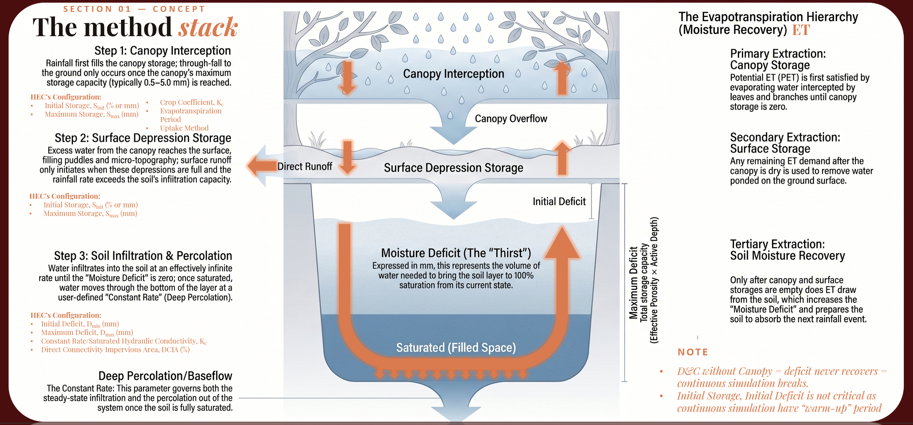
Figure 2 — Time-series concept
How D_init drains, how D_max caps the deficit, and when excess rainfall converts to runoff (deficit = 0).
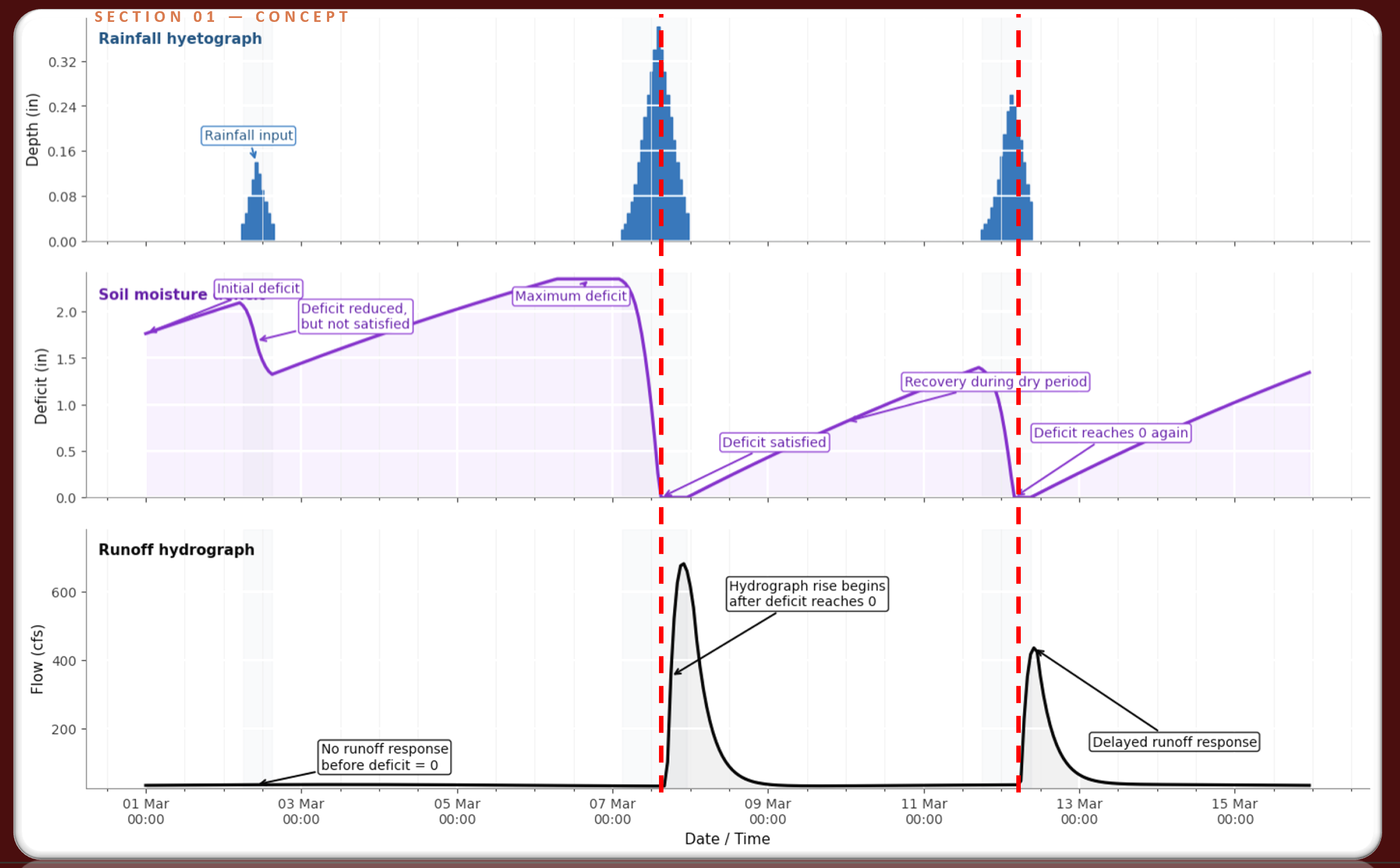
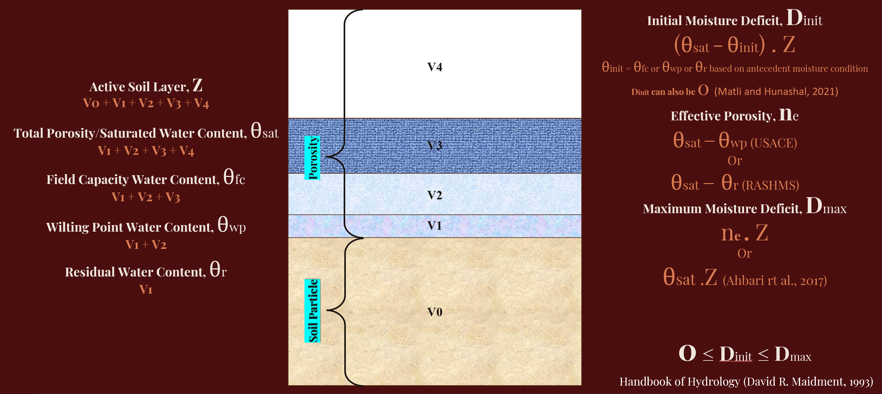
Figure 3 — Soil column + equations
Volumetric water-content fractions ( θsat , θfc , θwp , θr ) and the D_init / D_max formulations available in this tab. Maps directly onto the radio choices for Soil moisture data sources and D_max formula .
Rawls et al. (1982/1983) — HEC canonical
Soil moisture parameters from Rawls, Brakensiek & Saxton (1982); K_sat from Rawls, Brakensiek & Miller (1983) — Green-Ampt parameters. Always use Rawls 1983 for Constant Rate , not 1982 (1982 values are ~2× higher).
| Texture Class | θsat | θfc | θwp | θr | ne | K_sat 1982 (mm/hr) | K_sat 1983 (mm/hr) |
|---|---|---|---|---|---|---|---|
| Sand | 0.437 | 0.091 | 0.033 | 0.02 | 0.417 | 210.1 | 117.9 |
| Loamy Sand | 0.437 | 0.125 | 0.055 | 0.035 | 0.401 | 61.2 | 30 |
| Sandy Loam | 0.453 | 0.207 | 0.095 | 0.041 | 0.412 | 25.9 | 10.9 |
| Loam | 0.463 | 0.27 | 0.117 | 0.027 | 0.434 | 13.2 | 3.3 |
| Silt Loam | 0.501 | 0.33 | 0.133 | 0.015 | 0.486 | 6.9 | 6.6 |
| Sandy Clay Loam | 0.398 | 0.255 | 0.148 | 0.068 | 0.33 | 4.3 | 1.5 |
| Clay Loam | 0.464 | 0.318 | 0.197 | 0.075 | 0.39 | 2.3 | 1 |
| Silty Clay Loam | 0.471 | 0.366 | 0.208 | 0.04 | 0.432 | 1.5 | 1 |
| Sandy Clay | 0.43 | 0.339 | 0.239 | 0.109 | 0.321 | 1.3 | 0.5 |
| Silty Clay | 0.479 | 0.387 | 0.25 | 0.056 | 0.423 | 1 | 0.5 |
| Clay | 0.475 | 0.396 | 0.272 | 0.09 | 0.385 | 0.5 | 0.3 |
Note: Silt class is not in Rawls 1982 — when picked with this source, the app silently falls back to Silt Loam values.
Saxton & Rawls (2006) — pedotransfer functions
Updated dataset + organic matter effect; better fit for organic-rich soils. Includes Silt class (12 classes total).
| Texture Class | θsat | θfc | θwp | K_sat (mm/hr) |
|---|---|---|---|---|
| Sand | 0.46 | 0.1 | 0.05 | 108.1 |
| Loamy Sand | 0.46 | 0.12 | 0.05 | 96.7 |
| Sandy Loam | 0.45 | 0.18 | 0.08 | 50.3 |
| Loam | 0.46 | 0.28 | 0.14 | 15.5 |
| Silt Loam | 0.48 | 0.31 | 0.11 | 16.1 |
| Silt | 0.48 | 0.3 | 0.06 | 22 |
| Sandy Clay Loam | 0.43 | 0.27 | 0.17 | 11.3 |
| Clay Loam | 0.48 | 0.36 | 0.22 | 4.3 |
| Silty Clay Loam | 0.51 | 0.38 | 0.22 | 5.7 |
| Sandy Clay | 0.44 | 0.36 | 0.25 | 1.4 |
| Silty Clay | 0.52 | 0.41 | 0.27 | 3.7 |
| Clay | 0.5 | 0.42 | 0.3 | 1.1 |
Carsel & Parrish (1988) — van Genuchten parameters
Different framework (van Genuchten model fitting). Provides θr directly. Use for sensitivity / Monte Carlo analysis. Note: does NOT publish θfc or θwp — picking this source for those is blocked.
| Texture Class | θsat | θr | K_sat (mm/hr) |
|---|---|---|---|
| Sand | 0.43 | 0.045 | 297 |
| Loamy Sand | 0.41 | 0.057 | 145.9 |
| Sandy Loam | 0.41 | 0.065 | 44.2 |
| Loam | 0.43 | 0.078 | 10.4 |
| Silt Loam | 0.45 | 0.067 | 4.5 |
| Silt | 0.46 | 0.034 | 2.5 |
| Sandy Clay Loam | 0.39 | 0.1 | 13.1 |
| Clay Loam | 0.41 | 0.095 | 2.6 |
| Silty Clay Loam | 0.43 | 0.089 | 0.7 |
| Sandy Clay | 0.38 | 0.1 | 1.2 |
| Silty Clay | 0.36 | 0.07 | 0.2 |
| Clay | 0.38 | 0.068 | 2 |
HSG → CR fallback table
Used when texture data is unavailable. Two range sources: HEC TRM / Saleh et al. (2011) is narrower and conservative; Cahyono & Adidarma (2019) / Sahu et al. (2023) is wider for sensitivity check.
| HSG | Description | CR HEC TRM low | CR HEC TRM high | CR Cahyono low | CR Cahyono high |
|---|---|---|---|---|---|
| A | Deep, well-drained sands/gravels; low runoff potential | 7.62 | 11.43 | 36.1 | — |
| B | Moderately deep, well-drained; moderate infiltration | 3.81 | 7.62 | 14.5 | 36.1 |
| C | Layers impeding drainage; slow infiltration | 1.27 | 3.81 | 1.5 | 14.5 |
| D | High clay, shallow, or high water table; very slow | 0 | 1.27 | 0 | 1.5 |
USDA TR-55 Table 2-2a — % impervious by LULC class
Used as guidance when filling the per-LULC-class connected impervious fraction. Note: TR-55 % impervious is NOT the same as DCIA — multiply by a connectivity factor (0–1) to get the DCIA fraction.
| LULC class | % impervious |
|---|---|
| Open space / parks (good condition) | 0 |
| Residential 1 acre lots | 20 |
| Residential 1/2 acre lots | 25 |
| Residential 1/4 acre lots | 38 |
| Residential 1/8 acre lots (apartments) | 65 |
| Commercial / business | 85 |
| Industrial | 72 |
| Roads / streets / parking lots (paved) | 100 |
AMC selection — θ_init by antecedent condition
| Antecedent condition | θ_init | D_init result |
|---|---|---|
| During / just after saturating rain | θ_sat | 0 mm |
| ≥3 days after saturating rain | θ_fc | (θ_sat − θ_fc) × Z |
| End of dry season | θ_wp | (θ_sat − θ_wp) × Z = D_max (Option 1) |
| Extended drought | θ_r | (θ_sat − θ_r) × Z = D_max (Option 2) |
D_max formulation comparison
| Option | Formula | Source | Rationale |
|---|---|---|---|
| 1 (default) | (θ_sat − θ_wp) × Z | HEC-HMS tutorial; Sahu & Vidyarthi (2025) | Simple Canopy ET stops at θ_wp; nothing further dries the soil |
| 2 | (θ_sat − θ_r) × Z = n_e × Z | HEC TRM; RASHMS | Uses physical minimum (θ_r); more calibration headroom |
| 3 | θ_sat × Z | Ahbari et al. (2018) | Absolute upper bound; treats entire pore space as recoverable storage |
Always: Option 1 ≤ Option 2 ≤ Option 3 (because θ_r < θ_wp < θ_sat).
Calibration brackets — Option A / B / C
Three locked source-tables drive the min/max bracket columns on the Results sub-tab for Max Deficit (B.4) and Constant Rate (B.5). Engineer picks one via the radio on the User Defined sub-tab; the same radio drives Canopy and Surface tabs too. Initial Deficit and DCIA are not bracketed (D_init is a state variable, DCIA is GIS-derived).
B.4 — Max Deficit envelope per USDA texture (Option B, area-weighted)
( θsat − θwp ) × Z, Z ∈ [300, 1500] mm. θsat and θwp spread across Rawls 1982 + Saxton 2006.
| USDA texture | D_max min (mm) | D_max max (mm) | Source |
|---|---|---|---|
| Sand | 120 | 615 | Rawls 1982 + Saxton 2006 spread, Z 300–1500 mm |
| Loamy Sand | 115 | 615 | Rawls 1982 + Saxton 2006 spread, Z 300–1500 mm |
| Sandy Loam | 107 | 555 | Rawls 1982 + Saxton 2006 spread, Z 300–1500 mm |
| Loam | 96 | 519 | Rawls 1982 + Saxton 2006 spread, Z 300–1500 mm |
| Silt Loam | 111 | 555 | Rawls 1982 + Saxton 2006 spread, Z 300–1500 mm |
| Silt | 126 | 630 | Saxton 2006 (Silt only); Z 300–1500 mm |
| Sandy Clay Loam | 75 | 390 | Rawls 1982 + Saxton 2006 spread, Z 300–1500 mm |
| Clay Loam | 78 | 401 | Rawls 1982 + Saxton 2006 spread, Z 300–1500 mm |
| Silty Clay Loam | 79 | 435 | Rawls 1982 + Saxton 2006 spread, Z 300–1500 mm |
| Sandy Clay | 57 | 287 | Rawls 1982 + Saxton 2006 spread, Z 300–1500 mm |
| Silty Clay | 69 | 375 | Rawls 1982 + Saxton 2006 spread, Z 300–1500 mm |
| Clay | 60 | 305 | Rawls 1982 + Saxton 2006 spread, Z 300–1500 mm |
B.5 — Constant Rate envelope per USDA texture (Option B, area-weighted)
Max = Carsel & Parrish 1988 mean K_sat. Min = 0.3 × Rawls 1983 estimate (calibration reduction factor).
| USDA texture | CR min (mm/hr) | CR max (mm/hr) | Source |
|---|---|---|---|
| Sand | 32 | 297 | Max = Carsel & Parrish 1988 K_sat mean; Min = 0.3 × Rawls 1983 |
| Loamy Sand | 9 | 146 | Max = Carsel & Parrish 1988 K_sat mean; Min = 0.3 × Rawls 1983 |
| Sandy Loam | 3.3 | 50 | Max = Carsel & Parrish 1988 K_sat mean; Min = 0.3 × Rawls 1983 |
| Loam | 1 | 16 | Max = Carsel & Parrish 1988 K_sat mean; Min = 0.3 × Rawls 1983 |
| Silt Loam | 1.4 | 22 | Max = Carsel & Parrish 1988 K_sat mean; Min = 0.3 × Rawls 1983 |
| Silt | 0.8 | 22 | Max = Carsel & Parrish 1988 K_sat mean; Min = 0.3 × Rawls 1983 |
| Sandy Clay Loam | 0.5 | 13 | Max = Carsel & Parrish 1988 K_sat mean; Min = 0.3 × Rawls 1983 |
| Clay Loam | 0.3 | 4.3 | Max = Carsel & Parrish 1988 K_sat mean; Min = 0.3 × Rawls 1983 |
| Silty Clay Loam | 0.2 | 5.7 | Max = Carsel & Parrish 1988 K_sat mean; Min = 0.3 × Rawls 1983 |
| Sandy Clay | 0.2 | 1.4 | Max = Carsel & Parrish 1988 K_sat mean; Min = 0.3 × Rawls 1983 |
| Silty Clay | 0.1 | 3.7 | Max = Carsel & Parrish 1988 K_sat mean; Min = 0.3 × Rawls 1983 |
| Clay | 0.1 | 2 | Max = Carsel & Parrish 1988 K_sat mean; Min = 0.3 × Rawls 1983 |
Option A — HEC-HMS optimization defaults (scalar single envelope)
| Parameter | Min | Max | Source |
|---|---|---|---|
| Max Deficit (mm) | 0.001 | 1000 | HEC-HMS Technical Reference Manual |
| Constant Rate (mm/hr) | 0.001 | 300 | HEC-HMS Technical Reference Manual |
Option C — Calibrated literature ranges (scalar single envelope)
| Parameter | Min | Max | Min source | Max source |
|---|---|---|---|---|
| Max Deficit (mm) | 42.9 | 525.98 | Pudasaini et al. (2024) | Sahu & Vidyarthi (2025) |
| Constant Rate (mm/hr) | 0.01 | 6 | Kafle (2019) | Kherde et al. (2024) |
Calibrated values across reviewed studies
- Babu & Kumar (2024) — Chaliyar Kerala (tropical forest); ID=10, Dmax=100, CR=0.4, DCIA=0.2 (tropical humid benchmark)
- Sahu & Vidyarthi (2025) — Mahanadi India agricultural; ID=260–339, Dmax=463–526, CR=0.55, DCIA=17–19
- Madhushankha 2021 — Baddegama Sri Lanka 40% urban; ID=12.998, Dmax=50.483, CR=1.00, DCIA=40
- Pudasaini et al. (2024) — Kifissos Greece urban; ID=20% of Dmax, Dmax=42.9–108.9, DCIA=16.8–28
- Matli & Hunashal (2021) — Paravar India tropical; ID=0, Dmax=100, CR=1.32, DCIA=8
- Ahbari et al. (2018) / Moumni et al. (2021) — Morocco data-scarce; Dmax=654 or 81.8, CR=3.9 or 3.1, DCIA=0.4 or 7.7 (Ahbari uses Dmax = θ_sat × Z)
- USACE Tutorial — EF Russian River; ID=44.5 or 277, Dmax=178 or 277, CR=~1.0 or 0.5, DCIA=0
- Kafle (2019) — Koshi Nepal Himalayan; ID=4–6, Dmax=40–70, CR=0.01–1.3
- Kherde et al. (2024) — Tropical India agricultural; ID=80, Dmax=135, CR=6.0, DCIA=0
Citations
- Rawls, W. J., Brakensiek, D. L., & Saxton, K. E. (1982). Estimation of soil water properties. Transactions of the ASAE , 25(5), 1316–1320.
- Rawls, W. J., Brakensiek, D. L., & Miller, N. (1983). Green-Ampt infiltration parameters from soils data. Journal of Hydraulic Engineering , 109(1), 62–70.
- Saxton, K. E., & Rawls, W. J. (2006). Soil water characteristic estimates by texture and organic matter for hydrologic solutions. Soil Science Society of America Journal , 70(5), 1569–1578.
- Carsel, R. F., & Parrish, R. S. (1988). Developing joint probability distributions of soil water retention characteristics. Water Resources Research , 24(5), 755–769.
- USDA NRCS (1986). Urban Hydrology for Small Watersheds, TR-55 . USDA Natural Resources Conservation Service.
- Saleh, A., et al. (2011). HSG → K_sat ranges adopted in HEC Technical Reference Manual.
- Cahyono, B., & Adidarma, W. (2019); Sahu, M. K. et al. (2023) — wider HSG → K_sat ranges for sensitivity analysis.
- Shangguan, W., et al. (2017). Mapping the global depth to bedrock for land surface modeling. Journal of Advances in Modeling Earth Systems , 9(1), 65–88. [BDRICM raster source]
- Ross, C. W., et al. (2018). Global Hydrologic Soil Groups (HYSOGs250m) . ORNL DAAC. doi:10.3334/ORNLDAAC/1566. [HYSOGs250m raster source]
Compute the 12 monthly baseflow values per sub-basin via the
HP 11 (DID Malaysia 2018) regional power-law
Q_B = a · A^b
. Engineer picks the region; the
app pulls each sub-basin's area from the uploaded basin
shapefile and applies the matching coefficients. The same
Q_B is assigned to all 12 months (first-cut continuous
simulation per HP 11).
HP 11 region (DID Malaysia 2018)
Separation method
HP 11 region (for transfer exponent φ)
HP 11 (DID Malaysia 2018) — regional power-law
Q_B [m^3/s] = a · A^b for sub-basin area A in km^2. Coefficients were fit by DID Malaysia on hundreds of national gauges through 2017; three regional sets cover Peninsular Malaysia, Sabah, and Sarawak.
| Region | a | b | Equation |
|---|---|---|---|
| Peninsular Malaysia | 0.11 | 0.8589 | Q_B = 0.11 · A^0.8589 |
| Sabah | 0.0783 | 0.8653 | Q_B = 0.0783 · A^0.8653 |
| Sarawak | 0.0111 | 1.1682 | Q_B = 0.0111 · A^1.1682 |
Critical caveat — event-design baseline, not climatology
Per HP 11, Q_B is the average pre-storm baseflow sampled across flood events with dry-to-moderately-wet antecedent conditions. It is an event-design baseline , not the calendar-year mean baseflow. Applying the same Q_B to all 12 months is a first-cut continuous-simulation approximation — a last-resort fallback — defensible only for IDF / dam-safety studies where baseflow < 1% of peak. For genuine continuous simulation, prefer gauge- derived 12-month separation (planned Mode 2).
Inputs the app uses
-
Sub-basin polygon shapefile (uploaded on the Basin tab)
— area per sub-basin pulled via
sf::st_area(reprojected to EPSG:6933 equal-area when needed). - Basin ID column — re-uses the column picked on the Basin → Info & Configuration tab.
HEC-HMS unit convention
Constant Monthly accepts absolute flow values only (m^3/s in SI, cfs in US Customary) — there is no Discharge per Area input. HMS auto-converts between unit systems if the Basin Model unit system is later changed.
Mode 2 — Gauge-derived (per-station fan-out)
When the basin has loaded streamflow gauges (Catchment & Stream Delineation completed), Mode 2 derives the 12 monthly Q_B per sub-basin from the actual gauge record instead of HP 11 alone. The pipeline runs per-station: for each loaded gauge, hourly Q → daily mean → baseflow separation → 12 monthly means at the gauge. Each sub-basin then borrows its donor gauge's monthly values, scaled by the Modified DAR equation.
Transfer equation:
Q_B,i,m = Q_B,donor,m · (A_i / A_donor)^φ
.
φ is the HP 11 regional exponent (engineer picks region once).
Per DID Malaysia HP 11, HP 11 is applied as the SCALING
exponent (preserving the gauge's seasonal climatology) rather
than as the direct magnitude (which would produce a flat 12-month value).
Separation methods
- Dry-period averaging (default for Sabah). For each calendar month, average gauge Q on days where the previous N days had areal rainfall below threshold. Months with fewer than 3 dry samples fall back to the all-year median monthly Q. Şengül & Ispirli 2022.
- Lyne–Hollick recursive filter (1979). Low-pass filter applied 3 passes (iterated). Parameter α controls the filter cutoff (typical 0.925).
- Eckhardt two-parameter filter (2005). Recursive filter with aquifer-type ceiling BFI_max. Parameter a is the recession constant; BFI_max comes from the aquifer type radio.
Donor rule (hybrid)
Each sub-basin gets a donor gauge based on the gauged-catchment membership table (from Catchment & Stream Delineation):
- Exactly 1 catchment contains the sub-basin → that gauge is the donor (typical Outlet/Centroid 1:1 case).
- Multiple catchments contain it (Cumulative method, nested gauges) → nearest gauge by centroid-to-POI Euclidean distance among the containing gauges.
- No catchment contains it (ungauged tributary or downstream extension) → nearest gauge among all loaded gauges by centroid distance.
Engineer can override the donor per sub-basin in the Results DT's Donor column.
Mass-balance check (informational)
Per donor gauge, per month, the ratio of (Σ sub-basin Q_B / gauge Q_B) is reported. With the HP 11 exponent ≠ 1, this ratio is NOT 1 by design — small headwater sub-basins yield more per km² than the integrated gauge catchment. Per HEC-HMS Technical Reference, the Constant Monthly method does NOT enforce mass conservation; this report is informational only.
Citations
- DID Malaysia (2018). Hydrological Procedure No. 11: Design Flood Hydrograph Estimation for Rural Catchments in Malaysia . Department of Irrigation and Drainage, Ministry of Water, Land and Natural Resources, Putrajaya.
- US Army Corps of Engineers (2000). HEC-HMS Technical Reference Manual . Hydrologic Engineering Center, Davis, CA.
- Vogel, R. M., & Kroll, C. N. (1992, 1995). Regional geohydrologic-geomorphic relationships for the estimation of low-flow statistics. Water Resources Research , 28(9), 2451–2458.
- Şengül, S., & Ispirli, M. N. (2022). Assessment of SCS Curve Number and HEC-HMS Methods in a Mountainous Karstic Basin (Turkey). Water , 14(3), 384.
- Lyne, V., & Hollick, M. (1979). Stochastic time- variable rainfall-runoff modeling. In Proc. Hydrology and Water Resources Symposium , pp. 89–93. Institution of Engineers Australia.
- Eckhardt, K. (2005). How to construct recursive digital filters for baseflow separation. Hydrological Processes , 19(2), 507–515.
- Qamar, M. U., et al. (2025). Amalgamated Drainage Area Ratio and Nearest Neighbors approach for streamflow regionalization in British Columbia, Canada (preprint).
Configure Recession baseflow parameters per sub-basin:
Q₀
(initial discharge),
k
(recession constant), and
Threshold
. Model:
Q_t = Q₀ · kᵗ
.
Multi-sub-basin first-cut defaults: HP 11 power-law for Q₀,
k = 0.95 (humid-tropical GW), Ratio-to-Peak = 0.1.
Initial Discharge (Q₀) — derivation method
Recession constant (k)
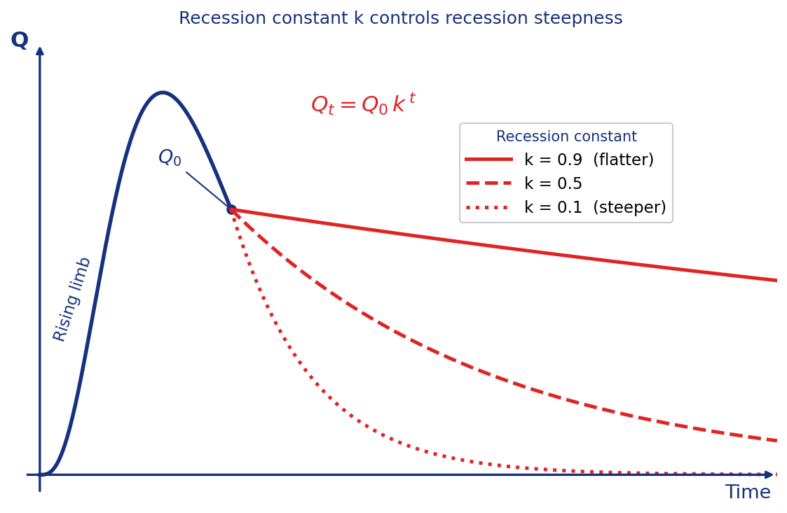
- Groundwater-dominated (rural humid tropical, deep soils) → 0.93–0.995
- Interflow-dominated (mixed catchments, intermediate decay) → 0.70–0.94
- Surface-runoff-dominated (urbanised, flashy, or shallow-soil) → 0.30–0.80
Threshold (recession turn-on flow)
Recession equation
Q_t = Q₀ · kᵗ
(linear exponential decay). HEC-HMS Recession is linear-only;
nonlinear storage-discharge (Aksoy & Wittenberg 2011) is a
separate 'Nonlinear Boussinesq' HMS method.
| Symbol | Meaning | Unit (SI) |
|---|---|---|
| Q0 | Initial discharge at start of recession | m³/s (or (m³/s)/km²) |
| k | Recession constant; Q₀/Q₁ ratio per day | dimensionless, 0 < k < 1 |
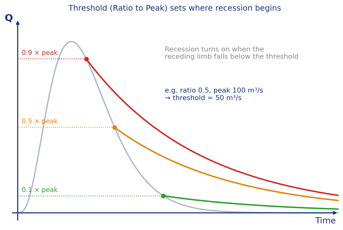
| Threshold | Flow at which the recession turns on | Ratio-to-Peak (0–1) OR Discharge (m³/s) |
HP 11 (DID Malaysia 2018) regional power-law
Used to derive Q₀ per sub-basin. Same equation set as the Constant Monthly tab's HP 11 reference; here it fits the event-design baseflow Q₀ role more cleanly than the Constant Monthly use case (HP 11 — event-design baseline).
| Region | a | b | Equation (Q₀ in m³/s, A in km²) |
|---|---|---|---|
| Peninsular Malaysia | 0.11 | 0.8589 | Q₀ = 0.11 · A^0.8589 |
| Sabah | 0.0783 | 0.8653 | Q₀ = 0.0783 · A^0.8653 |
| Sarawak | 0.0111 | 1.1682 | Q₀ = 0.0111 · A^1.1682 |
Literature k ranges (Linsley et al. 1982; Tallaksen 1995)
| Flow component | k (daily) | Notes |
|---|---|---|
| Groundwater | 0.93 – 0.995 | Slow decay; humid tropical typically 0.95+ |
| Interflow | 0.70 – 0.94 | Shallow subsurface, intermediate decay |
| Surface runoff | 0.30 – 0.80 | Rapid decay; rarely modelled with Recession |
Calibrated values — Malaysian / SE-Asian studies
| Study | Catchment | Q₀ | k | Threshold (type) |
|---|---|---|---|---|
| Hong et al. (2020) | Sg Melaka, Malaysia | 1.62 m³/s | 0.97 | 0.1 (Ratio) |
| Azli & Abdullah (2025) | Bandar Segamat, Malaysia | 0.5 m³/s | 0.5 | 50 m³/s (Discharge) |
| Gunathilake et al. (2020) | Seethawaka River, Sri Lanka | 12–30 m³/s | 0.60 | 0.01 (Ratio) |
| Nandalal & Ratnayake (2010) | Ellegawa, Sri Lanka | 65.0 m³/s | 0.90 | 0.05 (Ratio) |
| USACE Tutorial | Mahoning Creek, USA | 1.0 cfs/mi² | 0.6 | 0.4 (Ratio) |
Threshold guidance
- Ratio-to-Peak (recommended) — independent of basin size; defensible across multi-sub-basin models. Typical R = 0.1–0.5.
- Discharge — fixed flow; depends on sub-basin size, so calibrate per sub-basin if used.
Initial Type guidance
- Discharge per Area (recommended for multi-sub-basin) — uniform yield assumption is more defensible than uniform absolute discharge across sub-basins of different sizes.
- Discharge — useful when matching observed flow at a single gauge.
Critical caveats
- Mass NOT conserved — baseflow volume can exceed precipitation. Use Linear Reservoir if mass balance matters.
- One k cannot separate interflow from groundwater.
- Threshold sensitivity — do NOT transfer minor-flood parameters to extreme events.
- Recession does NOT affect flood peak; governs falling limb and volume only.
- Calibration order: k and Threshold are refined LAST, after CN + Time Lag (Yu & Zhang 2023).
Citations
- DID Malaysia (2018). Hydrological Procedure No. 11: Design Flood Hydrograph Estimation for Rural Catchments in Malaysia .
- US Army Corps of Engineers. HEC-HMS Technical Reference Manual — Recession Model .
- Hong, Y.M., Yap, M.K., et al. (2020). Application of HEC-HMS for streamflow infill in Sg Melaka, Malaysia.
- Azli, A. F., & Abdullah, J. (2025). Flood forecasting calibration in Bandar Segamat, Malaysia.
- Linsley, R. K., Kohler, M. A., & Paulhus, J. L. H. (1982). Hydrology for Engineers . McGraw-Hill.
- Tallaksen, L. M. (1995). A review of baseflow recession analysis. Journal of Hydrology , 165(1–4), 349–370.
- Vogel, R. M., & Kroll, C. N. (1996). Estimation of baseflow recession constants. Water Resources Management , 10(4), 303–320.
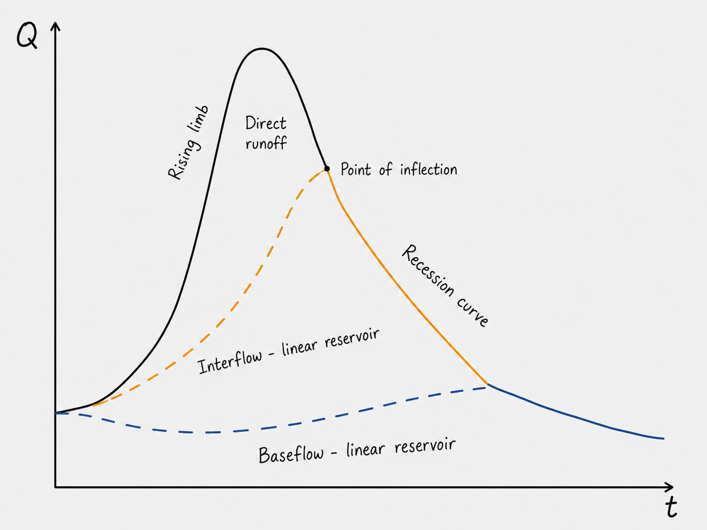
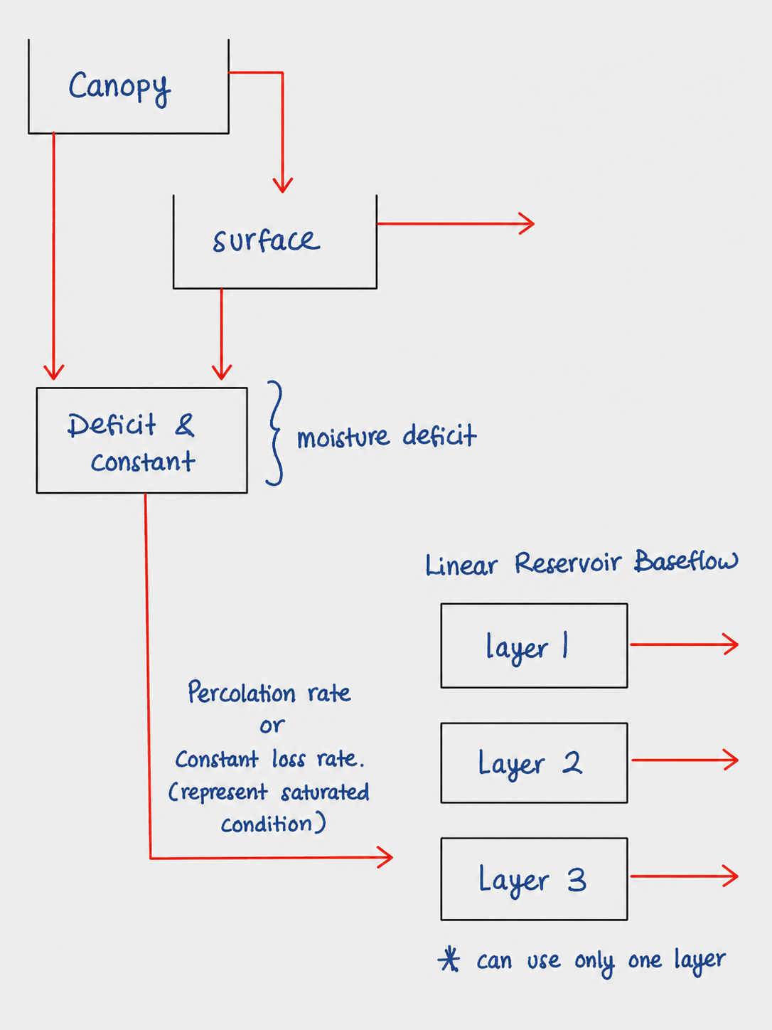
Configure Linear Reservoir baseflow per sub-basin. Each layer = an independent linear reservoir in PARALLEL; loss-method infiltration splits via Fraction. K is the storage time constant.
Number of GW layers
Initial Type (HEC-HMS native)
Initial value derivation method
GW Fraction (split of loss-method infiltration)
GW Reservoir count (Steps in cascade)
GW Coefficient (K, hours) - derivation
K_GWn = multiplier x R
;
R = ratio * Tc / (1 - ratio)
- 0.65 = HEC canonical (natural rural basin)
- 0.7 = flat and marshy
- 0.2-0.35 = natural basin with significant slope
- 0.1 = urbanised / steep
Calibration brackets
Seeds Min/Max columns in the Results table for all GW layers. Per-row overrides in the Results DT persist until a global changes here (nuclear reset).
Governing equations
dS/dt = I - O
;
S = K * O
=> outflow = storage / K => mass conserved (HEC Tech Ref).
Layers are in PARALLEL (Fractions split infiltration) ; Steps within a layer are in SERIES (cascade of reservoirs).
| Symbol | Meaning | Unit (SI) |
|---|---|---|
| K | Storage coefficient per layer | hours |
| Fraction | Share of loss-method infiltration to layer | dimensionless [0,1] |
| Steps | Linear reservoirs in series within a layer | integer >= 1 |
| Initial | Initial discharge in layer at t = 0 | m^3/s or (m^3/s)/km^2 |
| R | Clark Storage Coefficient (transform method) | hours |
| Tc | Time of concentration | hours (from Tc tab / 60) |
K derivation method
R = ratio * Tc / (1 - ratio)
;
K_GWn = mult_n * R
| Ratio R/(Tc+R) | Catchment type |
|---|---|
| 0.65 | HEC canonical default (natural rural) |
| 0.7 | Flat and marshy |
| 0.2-0.35 | Natural basin with significant slope |
| 0.1 | Urbanised / steep |
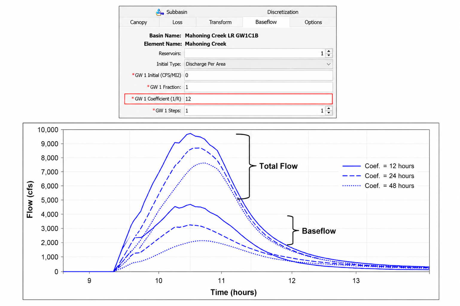
Effect of storage coefficient K on the baseflow recession.
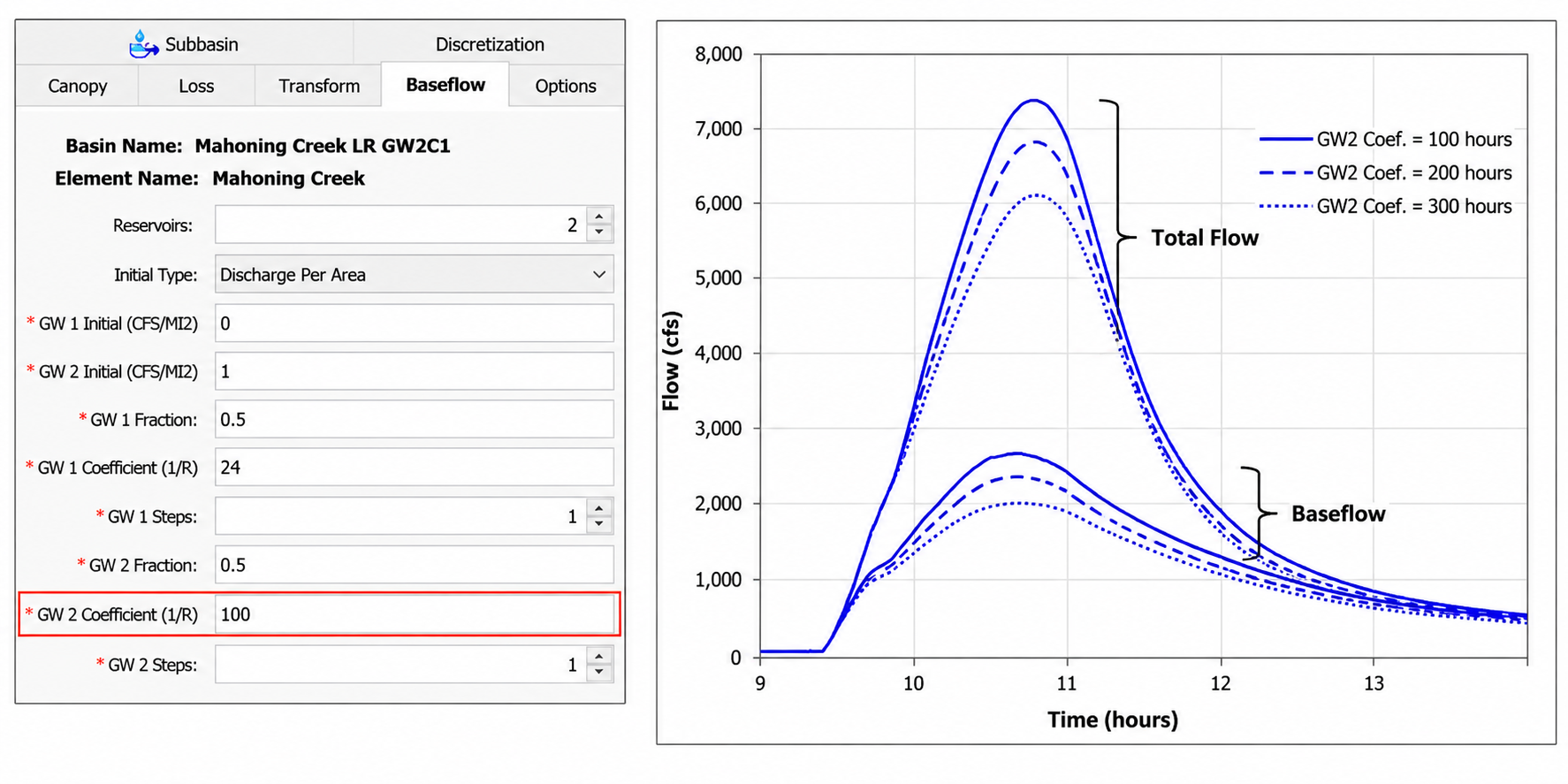
Effect of the GW2 storage coefficient on the baseflow shape.
Layer-purpose guide
| Layer | Models | Response | Typical K (hr) - Holberg 2015 Indiana proxy |
|---|---|---|---|
| GW1 | Interflow / shallow subsurface | Fastest | ~48-72 (range 34-85) |
| GW2 | Baseflow / shallow groundwater | Medium | ~250-500 (range 324-547) |
| GW3 | Deep groundwater | Slowest | > 1000 (extrapolated) |
Initial Discharge derivation methods
- Scalar default - 0 m^3/s (Discharge) or 0.01 (m^3/s)/km^2 (Discharge per Area). USACE Mahoning Creek tutorial.
- HP 11 power-law - Q0 = a * A^b per sub-basin; yield placed in slowest enabled layer (DID Malaysia 2018).
- Manual per sub-basin - engineer types values directly in Results DT.
| Region | a | b | Equation (Q0 m^3/s, A km^2) |
|---|---|---|---|
| Peninsular Malaysia | 0.11 | 0.8589 | Q0 = 0.11 * A^0.8589 |
| Sabah | 0.0783 | 0.8653 | Q0 = 0.0783 * A^0.8653 |
| Sarawak | 0.0111 | 1.1682 | Q0 = 0.0111 * A^1.1682 |
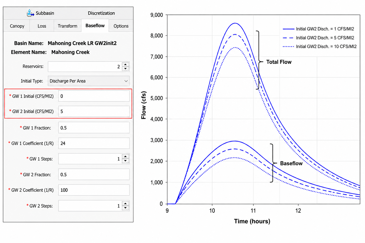
Effect of Initial Discharge on the hydrograph rising limb / pre-event baseflow.
Fraction + Steps guidance
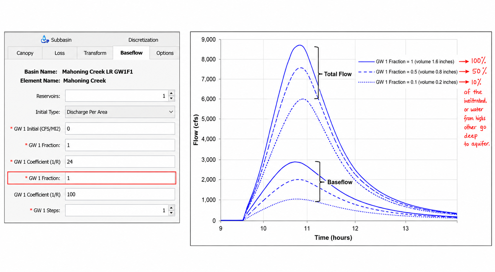
Effect of Fraction on the partitioned baseflow volume.
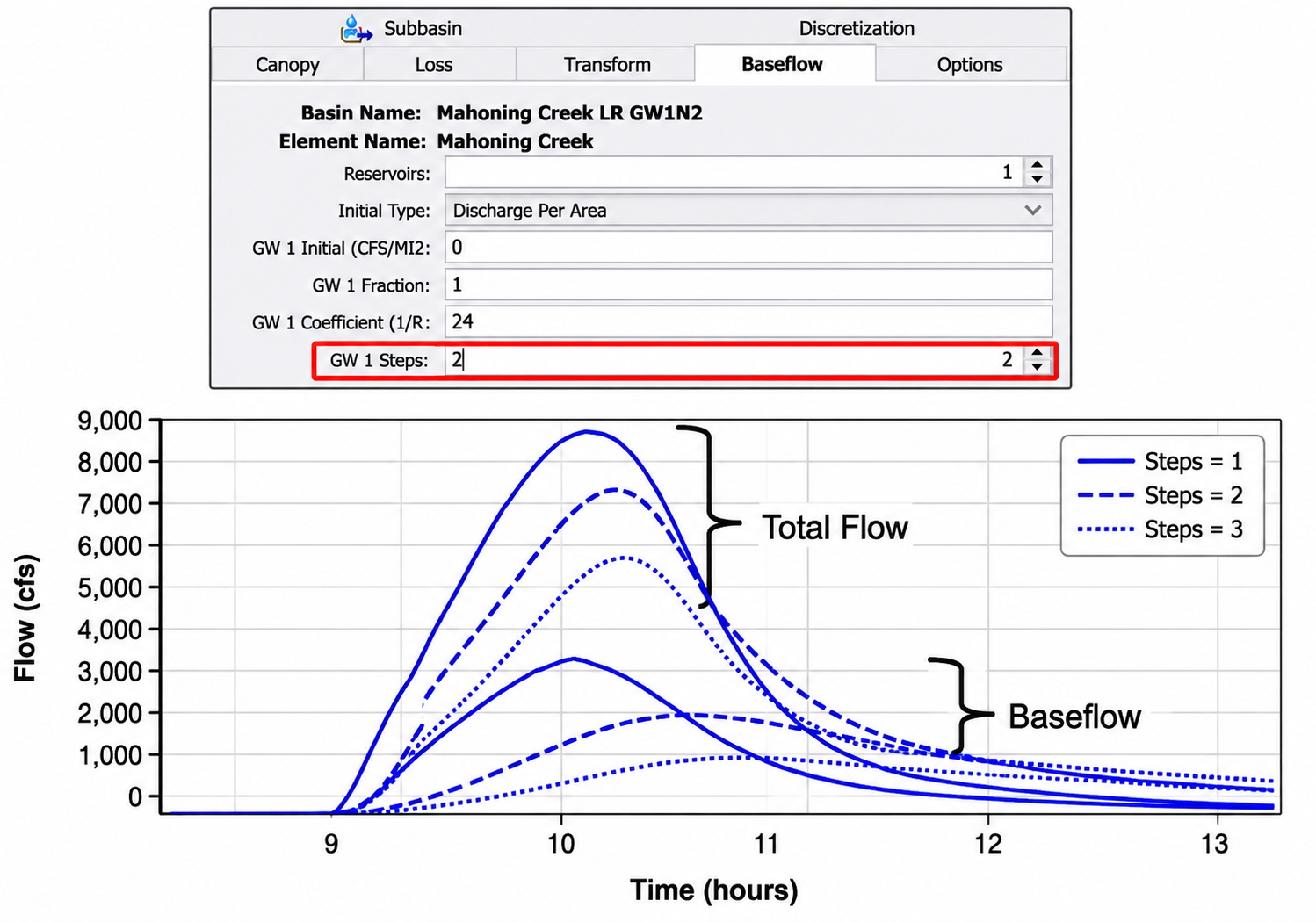
Effect of Steps (number of reservoirs in series within a layer) on the hydrograph timing/shape.
| n_layers | GW1 | GW2 | GW3 | Sum | Implication |
|---|---|---|---|---|---|
| 1 | 0.8 | - | - | 0.8 | 0.2 deep recharge |
| 2 | 0.5 | 0.5 | - | 1.0 | No deep recharge (humid-tropical canonical) |
| 3 | 0.4 | 0.4 | 0.2 | 1.0 | No deep recharge |
Critical caveats
- Mass IS conserved - unlike Recession + Constant Monthly. Annual volume not displayed because actual volume = function of loss-method infiltration at HEC-HMS runtime.
- Canonical loss-method pair - Deficit & Constant (passes only saturated losses; cleaner than CN/Green-Ampt which pass total infiltration including soil-bound water).
- Tc must be computed first - Run disabled until Tc tab returns results.
- No Sabah/Borneo LR published study — closest proxy: Attar et al. 2025 (Jhelum India, sub-humid temperate). Calibrate against outlet gauge BFI (target 0.50-0.75).
Sabah Papar starting points
| Param | GW1 (interflow) | GW2 (baseflow) | GW3 (deep, optional) | Basis |
|---|---|---|---|---|
| Initial Discharge | 0 | Q0,i / A_i (HP 11 Sabah per-area) | 0 (only if GW3 used) | HEC canonical |
| Fraction | 0.5 | 0.5 | 0 (or 0.2 if 3-layer) | HEC canonical humid-tropical |
| K (hours) | ~48-72 (3*R) | ~250-500 (10*R) | > 1000 (20*R extrapolation) | HEC Clark-multiplier rule |
| Steps | 1 | 1 | 1 | HEC functional minimum |
Further reading
- USACE HEC - Applying the Linear Reservoir Baseflow Method (Confluence canonical tutorial).
- USACE HEC - HEC-HMS Technical Reference Manual - Linear Reservoir Model .
- Matt Fleming (HEC Official, 2021) - L8c Linear Reservoir Baseflow (YouTube).
- Holberg, J.M. (2015). MS Thesis, Indiana University (SMA + LR coupling case study).
- Poudel & Vasconcelos (2026). Water 18(2), 182 (LR parameter sensitivity).
Citations
- DID Malaysia (2018). Hydrological Procedure No. 11 .
- USACE. HEC-HMS Technical Reference Manual - Linear Reservoir Model .
- USACE. Applying the Linear Reservoir Baseflow Method (Confluence tutorial).
- Attar, M.I., et al. (2025). Design storm estimation for flood risk assessment, Jhelum, India. Sci Rep .
- Holberg, J.M. (2015). A field investigation of channel-floodplain interaction and SMA in HEC-HMS (MS Thesis).
- Poudel & Vasconcelos (2026). Water 18(2), 182.
- Sengul & Ispirli (2022). Water 14(2), 284.
- Szilagyi (2018). LR routing stability (K > 0 => unconditionally stable).
- Maillet, E. (1905). Essai d'Hydraulique Souterraine et Fluviale (foundational LR; via Hall 1968).
- Nash, J.E. (1957). IAHS Publication 45 - cascade of linear reservoirs.
- Aksoy & Wittenberg (2011). Hydrol Sci J - nonlinear baseflow recession (limit-of-linearity caveat).
SCS dimensionless unit hydrograph. Pick Peak Rate Factor (Graph Type) and Lag source; per-row overrides are editable in the Results tab.
Clark unit hydrograph. Tc + R (Storage Coefficient). Method + Time-Area locked to Standard / Default per project scope.
Snyder synthetic unit hydrograph. Standard Lag (tp) + peaking coefficient Cp. HP 11 regional defaults pre-loaded.
Reach polylines have a digitized direction (first vertex -> last vertex). Downstream tabs assume upstream -> downstream. The app auto-detects via DEM elevation at the two endpoints; toggle any row that looks wrong on the map, then click Update Directions to commit + clear cross section results so they can be re-run with the corrected orientation.
Channel Manning's n method + per-reach Shape assignment. Pick Canonical Lookup for category-based ranges or Schneider Additive to build n from bed material + irregularity + obstructions + vegetation + meander. Default = Canonical Lookup, Natural main channel, Clean straight no pools.
Channel Manning's n method
Per-reach configuration Edit Shape, Channel n category, or the final n value directly. Eight Point and the relevant shape sub-tabs appear above as reaches are assigned.
Transect placement + 8-point extraction. Default station = reach midpoint, default length = 200 m, default sample count = 100 along the transect. Engineer can drag the station point on the Reach Map (unlock first), then click Run to regenerate only the moved transects.
On Run, the Basin Map shows the perpendicular transect lines. Only reaches whose station point was moved (or newly assigned) are re-extracted.
Eight-point coordinates Edit station or elevation directly in the table. Changes sync with the plot once Save Changes is clicked.
Pair each reach with a surveyed cross section. Run becomes active once a reach shapefile, DEM, and at least one surveyed XS are loaded. Edits made here do NOT change the original data under the Surveyed Cross Section tab.
Reach ↔ Surveyed XS pairing Click a row to view + edit that reach's cross section below. Use the Surveyed ID dropdown to change the pairing.
Left and Right overbank Manning's n per reach. Default = Canonical Lookup, Floodplain / overbank, Dense grass / turf. Pick Schneider Additive to build n from component tables. Left and Right are picked independently - cover often differs side-to-side.
Overbank Manning's n method
Right overbank
Mapping of Reach ID -> Cross Section ID + Left/Right Manning's n + Invert. Cross Section column is editable via dropdown; engineer can reuse one cross-section for multiple reaches when geometry is similar.
Per-reach Diameter (m) + Invert (m). Visible whenever any reach is assigned the Circle shape on the User Defined tab.
Per-reach Width (m) + Invert (m). Visible whenever any reach is assigned the Rectangular shape on the User Defined tab.
Per-reach Bottom Width (m) + Side Slope + Invert (m). Visible whenever any reach is assigned the Trapezoidal shape on the User Defined tab.
Combined per-reach result table - pulls Channel Manning's n from User Defined, Shape from User Defined, Cross Section ID from Eight Point Summary, Length and Slope from reach geometry. Initial Type = Discharge = Inflow, Space-Time = Auto DX Auto DT, Index Celerity defaults to 1.5 m/s (engineer can edit).
Canonical Lookup - Channel Manning's n
Source: Chow (1959), Barnes (1967), Arcement & Schneider (1989), EM 1110-2-1417. Use Barnes plates or Schneider Additive build-up to pin a defended single value within a range.
| Category | Description | n min | n max | Source |
|---|---|---|---|---|
| Natural main channel | Clean, straight, no pools | 0.025 | 0.033 | Chow 1959; Barnes 1967 |
| Natural main channel | Winding, some pools, clean | 0.033 | 0.045 | Chow 1959; Barnes 1967 |
| Natural main channel | Weedy, deep pools, some brush | 0.05 | 0.08 | Chow 1959; Arcement & Schneider 1989 |
| Natural main channel | Very weedy, heavy brush/timber | 0.075 | 0.15 | Chow 1959; Arcement & Schneider 1989 |
| Constructed / lined | Finished concrete | 0.011 | 0.015 | Chow 1959 |
| Constructed / lined | Unfinished concrete | 0.014 | 0.02 | Chow 1959 |
| Constructed / lined | Gravel / clean earth | 0.022 | 0.03 | Chow 1959 |
| Constructed / lined | Asphalt | 0.013 | 0.016 | Chow 1959; EM 1110-2-1417 |
Canonical Lookup - Floodplain / overbank Manning's n
Pick Left and Right overbank independently. Floodplain n is typically an order of magnitude above channel n; vegetation (n4) dominates.
| Category | Description | n min | n max | Source |
|---|---|---|---|---|
| Floodplain / overbank | Pasture, short grass | 0.03 | 0.05 | Chow 1959; Arcement & Schneider 1989 |
| Floodplain / overbank | Dense grass / turf | 0.1 | 0.48 | EM 1110-2-1417 (Tbl 7-1) |
| Floodplain / overbank | Scattered brush, dense shrubs | 0.05 | 0.15 | Arcement & Schneider 1989 |
| Floodplain / overbank | Heavy timber, dense underbrush | 0.1 | 0.2 | Arcement & Schneider 1989 |
Schneider Additive - components
Channel formula: n = (nb + n1 + n2 + n3 + n4) × m. Overbank formula drops n2 (no XS variation) and m (no sinuosity overland): n = nb + n1 + n3 + n4. Source: Arcement & Schneider (1989) USGS WSP 2339, Cowan (1956).
nb – bed material
| Category | Description | Value |
|---|---|---|
| Soil (firm) | Firm soil bed | 0.02 |
| Rock cut | Bedrock cut channel | 0.025 |
| Gravel (soft/fine) | Fine gravel substrate | 0.024 |
| Gravel (rough/coarse) | Coarse / cobble gravel substrate | 0.028 |
n1 – surface irregularity
| Category | Description | Value |
|---|---|---|
| Smooth | No bank surface irregularity | 0 |
| Minor | Slight bank irregularity | 0.005 |
| Moderate | Moderate bank irregularity (eroded, sloughed) | 0.01 |
| Severe | Severe bank irregularity (badly sloughed, jagged) | 0.02 |
n2 – cross-section variation (channel only)
| Category | Description | Value |
|---|---|---|
| Gradual | Cross-section size gradual | 0 |
| Occasional | Occasional XS shape change | 0.005 |
| Frequent (alternating) | Frequent alternating XS shape (vault range 0.010-0.015, midpoint used) | 0.0125 |
n3 – obstructions
| Category | Description | Value |
|---|---|---|
| Negligible | No notable obstructions | 0 |
| Minor | Minor (some debris, occasional boulders) | 0.0125 |
| Appreciable | Appreciable (notable debris jam, boulders, piers) | 0.025 |
| Severe | Severe (heavy jam, buildings, large boulders) | 0.05 |
n4 – vegetation
| Category | Description | Value |
|---|---|---|
| Low | Sparse vegetation (low) | 0.0075 |
| Medium | Moderate weeds / scattered brush | 0.0175 |
| High | Heavy grass / dense brush | 0.0375 |
| Very high | Dense brush + small trees / submerged willows | 0.075 |
m – meander / sinuosity correction (channel only)
| Category | Description | Value |
|---|---|---|
| Minor sinuosity (1.0-1.2) | Sinuosity ratio between 1.0 and 1.2 | 1 |
| Appreciable sinuosity (1.2-1.5) | Sinuosity ratio between 1.2 and 1.5 | 1.15 |
| Severe sinuosity (>1.5) | Sinuosity ratio greater than 1.5 | 1.3 |
Citations
- Chow, V. T. (1959). Open-Channel Hydraulics. McGraw-Hill, New York.
- Barnes, H. H. (1967). Roughness Characteristics of Natural Channels. USGS Water-Supply Paper 1849.
- Cowan, W. L. (1956). Estimating Hydraulic Roughness Coefficients. Agricultural Engineering, 37(7), 473-475.
- Arcement, G. J., & Schneider, V. R. (1989). Guide for Selecting Manning's Roughness Coefficients for Natural Channels and Flood Plains. USGS Water-Supply Paper 2339.
- USACE EM 1110-2-1417. Flood-Runoff Analysis. Engineer Manual, US Army Corps of Engineers.
Upload one or more Excel workbooks. Each sheet is treated as a single chainage cross section. Sheets named Sheet1 and empty sheets are skipped. Pick the EPSG of the surveyed Easting/Northing. Click any row below to plot that chainage's surveyed cross section overlaid with the DEM cross section extracted at the same Easting/Northing points.
Use the polyline tool on the Reach Map (left panel) to draw any line. The app samples the uploaded DEM along that line and renders an elevation profile here. Hover the plot to see the linked point on the map. Clear button wipes the drawn line.